db <- foreign::read.spss(file=paste0(getwd(),
                "/data/1186_Selects2019_CandidateSurvey_Data_v1.1.0.sav"),
                use.value.labels = T,
                to.data.frame = T)
sel <- db |>
  dplyr::select(B12,T9a) |>
  stats::na.omit() |>
  dplyr::rename("budget"="B12", "party_list"="T9a") |>
  plyr::mutate(budget=as.numeric(as.character(budget))) |>
  plyr::mutate(party_list=as.factor(party_list))
# filter candidates with maximally a budget of 100'000
boxplot(sel$budget)(M)AN(C)OVA presentation
Learn what (M)AN(C)OVA is and how to run the analysis in R
1 ANOVA: general logic
1.1 ANOVA purpose
ANOVA compares the distribution of values on a quantitative variable (central tendency, dispersion) for different sub-populations (different categories of the categorical independent variable)
Regression analysis: “The bigger X, the bigger Y”
- Relationships between two variables
- Metric independent variables
- Useful to evaluate survey data
Analysis of variance: “More in group A than in group B”
- Differences between two or more groups
- Categorical independent variables
- Useful for evaluating experimental data
1.2 Same logic: general linear model and F-test
Regression: The quality of the model results from the deviation of the individual values from the regression line
ANOVA: Model quality results from the deviation of the individual values from the group mean
If you want to compare the means of two groups, you can do a t-test.
If you want to compare the means of more than two groups, one would have to compare each group with each other.
2 Error components
2.1 Variation between and within groups
To see if the two variables are independent or if there is a relationship between them, we compare:
- variation between groups (central tendency: averages)
- variation within groups (dispersion: standard deviation)
There is a relationship between two variables when the different groups are distinct and homogeneous.
2.2 Variance decomposition
2.3 Total sum of squares (TSS)
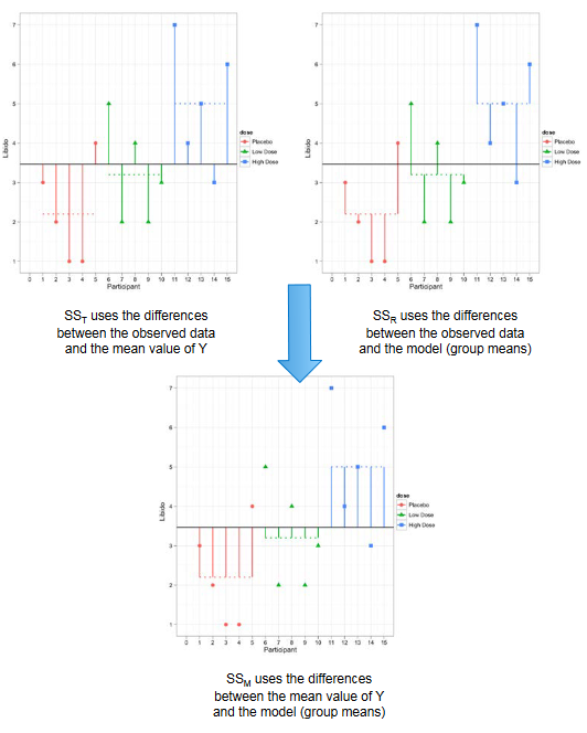
The total amount of variation within our data is the difference between each observed data point (\(\hat{y}_{ij}\)) and the grand mean (\(\hat{y}_{Grand}\)). We then square these differences and add them together to give us the total sum of squares (TSS).
\[ TSS = \sum{(\hat{y}_{ij} - \hat{y}_{Grand})^2} \]

2.4 Model sum of squares (MSS)
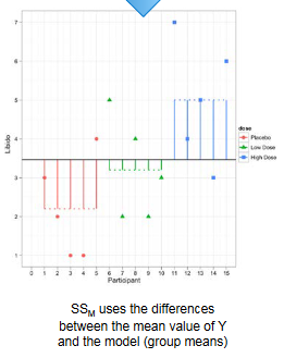
The model sum of squares (MSS) requires us to calculate the differences between each participant’s predicted value (\(\hat{y}_j\)) and the grand mean (\(\hat{y}_{Grand}\)). It is the sum of the squared distances between what the model predicts for each data point (i.e., the dotted horizontal line for the group to which the data point belongs) and the overall mean of the data (the solid horizontal line).
\[ MSS = \sum{n_j(\hat{y}_j - \hat{y}_{Grand})^2} \]
2.5 Residual sum of squares (SSE)
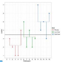
The final sum of squares is the residual sum of squares (SSE), which tells us how much of the variation cannot be explained by the model. The simplest way to calculate SSE is to subtract MSS from TSS. It is calculated by looking at the difference between the score obtained by a person and the mean of the group to which the person belongs.
\[ SSE = \sum{(y_{ij} - \hat{y}_i)^2} \]
2.6 Mean Squares (MS)
Sum of squares depend on the number of groups and the number of cases per group. MS are variances calculated by dividing the SS by the corresponding number of degrees of freedom.
- Model Mean Sum of Squares: \(MS_M = \frac{MSS}{df_M}\), \(df_M = k-1\).
- Mean sum of squares of the residuals: \(MS_R = \frac{RSS}{df_R}\), \(df_R = k(n_j-1) = n-k\).
The test variable \(F_{Ratio}\) is calculated from MS: \(F = \frac{MS_M}{MS_R}\).
3 ANOVA: statistical significance and strength of the relationship
4 Hypothesis test
Determine the statistical significance of the relationship (generalization to the population):
- H0: the two variables are independent
- H1: the two variables are dependent
Acceptance of H0 if p-value > 0.05 and of H1 if p-value < 0.05.
4.1 Strength of the relationship
Determine the strength of the relationship between the variables using the measure of association Eta (\(\eta\)):
- 0 = perfect independence
- 1 = perfect association
\(\eta^2\) informs us about the explanatory power of the model. It can be interpreted as the percentage of the variance of the DV explained by the IV.
4.2 Effect size: \(\eta^2\) and \(R^2\)
\(\eta^2\) is a measure of effect size that is commonly used in ANOVA models. It measures the proportion of variance associated with each main effect and interaction effect in an ANOVA model.
\[ \eta^2 =\frac{SS_{effect}}{SS_{total}} \]
where \(SS_{effect}\) is the sum of squares of an effect for one variable and \(SS_{total}\) is the total sum of squares in the ANOVA model.
The value for \(\eta2\) ranges from 0 to 1, where values closer to 1 indicate a higher proportion of variance that can be explained by a given variable in the model.
\(R^2\) gives the effect size of the entire model: proportion of variance (TSS) that can be explained by the model (MSS).
\[ R^2 = \frac{MSS_{overall}}{TSS} \]
5 Empirical exemple in R
5.1 Example
Let’s prepare data to investigate whether the campaigning budget varies significantly across parties:

5.2 Group means (and sd)
sel |> dplyr::group_by(party_list) |>
  dplyr::summarise(dplyr::across(.cols = budget,
                                 list(n = length,
                                      mean = mean,
                                      sd = sd)))
# A tibble: 8 × 4
party_list budget_n budget_mean budget_sd
<fct> <int> <dbl> <dbl>
1 FDP/PLR - The Liberals 186 13059. 21762.
2 CVP/PDC - Christian Democratic People's Party 319 5467. 12962.
3 SP/PS - Social Democratic Party 285 5626. 11580.
4 SVP/UDC - Swiss People's Party 170 6711. 15477.
5 GPS/PES - Green Party 246 4357. 10970.
6 GLP/PVL - Green Liberal Party 223 4297. 10668.
7 Other party 438 3534. 9455.
8 No party 23 5113. 12066.5.3 Recoding
Let’s recode the parties into fewer categories:
sel$party_list <- gsub(" -.*","",sel$party_list)
sel$lcr <- ifelse(sel$party_list=="SP/PS" |
                    sel$party_list=="GPS/PES", "left", NA)
sel$lcr <- ifelse(sel$party_list=="GLP/PVL" |
                    sel$party_list=="CVP/PDC", "center", as.character(sel$lcr))
sel$lcr <- ifelse(sel$party_list=="SVP/UDC" |
                    sel$party_list=="FDP/PLR", "right", as.character(sel$lcr))
table(sel$lcr)
center   left  right
   542    531    356
5.4 ANOVA and Eta
              Df    Sum Sq   Mean Sq F value   Pr(>F)
lcr            2 6.726e+09 3.363e+09   17.23 4.03e-08 ***
Residuals   1426 2.783e+11 1.952e+08
---
Signif. codes:  0 '***' 0.001 '**' 0.01 '*' 0.05 '.' 0.1 ' ' 1
461 observations deleted due to missingness- The p-value associated with the F-test is statistically significant (<0.05). Thus, there is a difference in the campaign budget between the different groups.
- The independent variable (party_list) explains 2.3% of the variance of the dependent variable (budget).
- A significant p-value implies that some of the group means are different in a one-way ANOVA test. But we don’t know which pairs of groups are different.
5.5 Multiple pairwise comparisons
We can compute Tukey Honest Significant Differences for doing numerous pairwise comparisons between the means of groups because the ANOVA test is significant.
  Tukey multiple comparisons of means
    95% family-wise confidence level

Fit: aov(formula = budget ~ lcr, data = sel)

$lcr
                  diff       lwr      upr     p adj
left-center    51.8473 -1949.525 2053.220 0.9979654
right-center 5041.6591  2805.573 7277.745 0.0000004
right-left   4989.8118  2744.563 7235.061 0.0000006
6 Assumptions
6.1 Variance homogeneity
To assume that the variances are homogeneous, there should be no clear correlations between residuals and fitted values (the mean of each group) in the plot below.
Levene’s test is recommended since it is not very sensitive to deviations from normal distribution. If the p-value is less than the significance level of 0.05, it indicates that the variance across groups is statistically significant.
Levene's Test for Homogeneity of Variance (center = median: sel)
        Df F value    Pr(>F)
group    7  9.8826 3.696e-12 ***
      1882
---
Signif. codes:  0 '***' 0.001 '**' 0.01 '*' 0.05 '.' 0.1 ' ' 1
An alternative approach (e.g., the Welch one-way test) does not necessitate the use of equal variance assumptions (in R: oneway.test() and pairwise.t.test())
6.2 Normality
We can infer normality if all of the points lie roughly along this reference line.
Run Shapiro-Wilk test on the ANOVA residuals. If the p-value is <0.05, it suggests that there is evidence of normality violation.
    Shapiro-Wilk normality test

data:  aov_residuals
W = 0.53433, p-value < 2.2e-16
The Kruskal-Wallis rank-sum test is a non-parametric alternative to one-way ANOVA that can be employed when the ANOVA assumptions are not met (in R: kruskal.test()).
7 Interaction hypothesis
7.1 Effect of two or more factors
To compare the influence of several different factors, it is necessary to test the interaction hypotheses: influence of a factor depending on one or more other factors (A and B).
- \(MSS_A\): Calculation with the groups of the factor A (we pretend that B does not exist)
- \(MSS_B\): Calculation with the groups of the factor B (we pretend that A does not exist)
- \(MSS_{AB}\): \(MSS-MSS_A-MSS_B\) indicates what the model can explain beyond factors A and B.
7.2 F score for multiple factors
A separate F is used for each factor and interaction term:
- Factor A: \(F = \frac{MS_{MA}}{MS_R}\)
- Factor B: \(F = \frac{MS_{MB}}{MS_R}\)
- Interaction AxB: \(F = \frac{MS_{MAB}}{MS_R}\)
7.3 Effect size: \(R^2\) and partial \(\eta^2\)
\(R^2\) gives the effect size of the entire model: proportion of variance (TSS) that can be explained by the model (MSS).
\[ R^2 = \frac{MSS_{overall}}{TSS} \]
Partial \(\eta^2\) is the respective effect size of the individual factors: reflect the proportion of the variance (TSS) that can be explained by the respective factors or interaction terms (SS effect).
- \(\eta^2\) for factor A: \(\frac{SS_A}{TSS}\)
- \(\eta^2\) for factor B: \(\frac{SS_B}{TSS}\)
- \(\eta^2\) for interaction AxB: \(\frac{SS_{AB}}{TSS}\)
The value for \(\eta^2_{partial}\) ranges from 0 to 1, where values closer to 1 indicate a higher proportion of variance explained by a given variable in the model after accounting for variance explained by other variables in the model.
8 Types of interaction
8.1 Typology
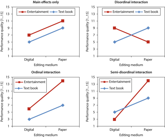
- null interaction: effects of factor A on the dependent variable are therefore the same at all stages of the factor B (parallel lines)
- ordinal interaction: effects of A are not the same at all factor levels of B (lines do not run parallel but do not cross)
- disordinal interaction: crossing lines (any main effects that may be present must not be interpreted)
- semi-disordinal: crossing lines or lines that do not cross (only one of the main effects that may be present may be interpreted)
9 Empirical exemple in R
9.1 Example
Let’s prepare data to investigate whether intention to participate in election depends on news consumption and party closeness:
db <- foreign::read.spss(file=paste0(getwd(),
                "/data/1184_Selects2019_Panel_Data_v4.0.sav"),
                use.value.labels = T,
                to.data.frame = T)
sel <- db |>
  dplyr::select(W1_f13400a, W1_f13400b,
                W1_f13400c, W1_f13400d,
                W1_f13400e, W1_f13400f,
                W1_f14000,
                W1_f10800) |>
  stats::na.omit() |>
  dplyr::rename("particip"="W1_f10800",
                "party"="W1_f14000") |>
  plyr::mutate(particip=as.numeric(particip))
sel$particip <- (sel$particip-5)*(-1) # reverse the scale
9.2 Create score of political news attention
# recode into 'high', 'medium' and 'low'
sel$newsatt_r = NA
sel$newsatt_r <- ifelse((sel$newsatt>=1.5 &
sel$newsatt<=2.5), "2. medium",
as.character(sel$newsatt_r))
sel$newsatt_r <- ifelse((sel$newsatt<1.5 &
is.na(sel$newsatt_r)), "1. low",
as.character(sel$newsatt_r))
sel$newsatt_r <- ifelse((sel$newsatt>2.5 &
is.na(sel$newsatt_r)), "3. high",
as.character(sel$newsatt_r))
table(sel$newsatt_r)
   1. low 2. medium   3. high
      738      4791      1091
9.3 Example of ordinal interaction
The main effects and the interaction effect are significant:
                  Df Sum Sq Mean Sq F value   Pr(>F)
newsatt_r          2    445  222.50 427.550  < 2e-16 ***
party              1    237  237.16 455.717  < 2e-16 ***
newsatt_r:party    2      8    4.01   7.698 0.000458 ***
Residuals       6614   3442    0.52
---
Signif. codes: 0 '***' 0.001 '**' 0.01 '*' 0.05 '.' 0.1 ' ' 110 Quiz
10.1 Can I answer these questions?
function quizInput({ questions, options}) {
let answers = questions.map(() => null);
let root = htl.html`<div
style="
display: grid;
grid-template-columns: 10% 10% 70% 10%;"
>
${options.map(
(opt) => htl.html`<div style="font-weight: bold">${opt}</div>`
)}
<div style="font-weight: bold">Statements</div>
<div style="font-weight: bold"></div>
${Array.from(questions.entries(), ([i, [question, correct]]) =>
quizInputRow({
question,
options,
correct,
onChange: (newAnswer) => {
answers[i] = newAnswer;
root.value = answers;
root.dispatchEvent(new CustomEvent("input"));
}
})
)}
</div>`;
root.value = answers;
return root;
}
function quizInputRow({
question,
options,
correct,
onChange = () => {}
}) {
let root = htl.html`<div>`;
function setAnswer(answer, initial = false) {
morph(
root,
htl.html`<div style="display: contents">
<form style="display: contents">
${options.map(
(opt) =>
htl.html`<label> </label>
<input
name=${question}  
type="radio"
value="${opt}"
checked=${opt === answer}
onChange=${() => setAnswer(opt)}
>
</input>`
)}
</form>
<div>${question}</div>
<div>   ${
answer === null ? "" : answer === correct ? "🟢" : "🔴"
}</div>
</div>`
);
root.value = answer;
if (!initial) {
root.dispatchEvent(new CustomEvent("input"));
onChange(answer);
}
}
setAnswer(null, true);
return root;
}
morph = require("https://bundle.run/nanomorph@5.4.2")True or false?
MC_1_1 = [
    ["The F-test in ANOVA helps prevent alpha error cumulation by checking if at least two groups differ significantly from each other", "true"],
    ["A significant p-value in an ANOVA test implies that all group means are different", "false"],
    ["An significant ordinal interaction in ANOVA suggests that the effects of one factor are not the same at all levels of the other factor", "true"],
    ["The measure of association Eta (η) in ANOVA ranges from 0 to 1, where values closer to 1 indicate a higher proportion of variance explained by the independent variable", "true"]
]

viewof answers_1_1 = quizInput({
  questions: MC_1_1,
  options: ["true", "false"]
})

Punkte_1_1 = {
const Sum =
    (answers_1_1[0] == MC_1_1[0][1])*1 +
    (answers_1_1[1] == MC_1_1[1][1])*1 +
    (answers_1_1[2] == MC_1_1[2][1])*1 +
    (answers_1_1[3] == MC_1_1[3][1])*1

var Punkte_1_1 = Sum - 2
if (Punkte_1_1 < 1) {Punkte_1_1 = 0}
return(Punkte_1_1)
}
Score:
11 ANCOVA
11.1 ANCOVA: definition and application
- ANCOVA is an analysis of covariance.
- It is used to measure the main effect and interaction effects of categorical variables on a continuous dependent variable while controlling the effects of selected other continuous variables which co-varies with the dependent variable.
Example: What is the effect of political affiliation on campaign budget while controlling for age of the candidate?
11.2 ANCOVA logic
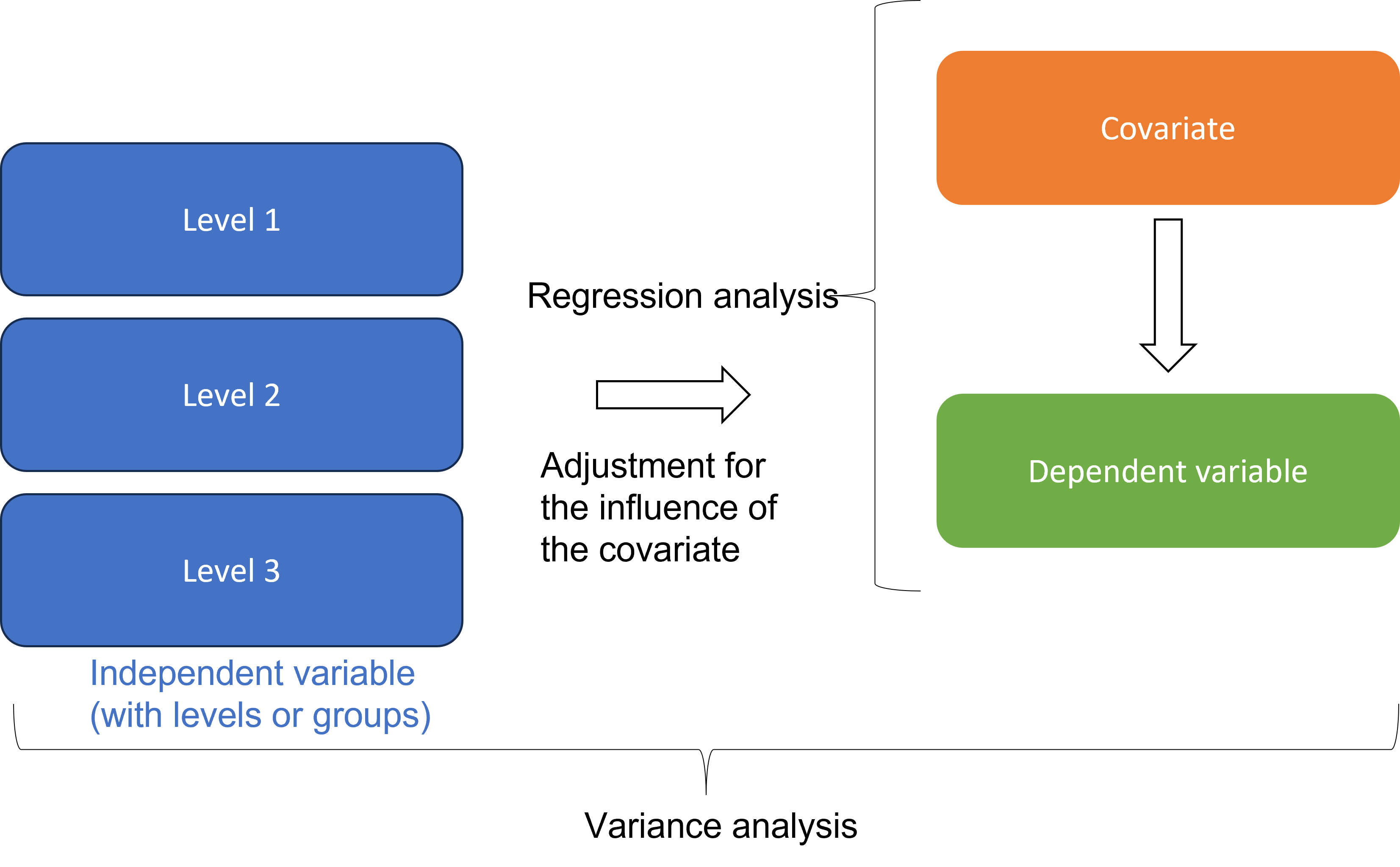
11.3 Usefulness of covariate(s)
Covariates help us with reducing unexplained variance and within-group variance (SSE).
The effect of the factors on the dependent variable can thus be determined more accurately (MSS).
This improves the explanatory power of the overall model (\(R^2\)).
The explanatory power of the factors (\(\eta^2\)) also improves.
11.4 Disadvantages
The strict cause-and-effect logic of an experimental design does not apply to covariates.
Futhermore, covariates must have a measurement (and they must be scale).
Moreover, one can never include all relevant covariates.
Note: We lose one degree of freedom of the residuals per covariate (SSE).
11.5 ANCOVA assumptions
- Assumption 1: Linearity between the covariate and the dependent variable at each level of the grouping variable.
- Assumption 2: Homogeneity of regression slopes: the slopes of the regression lines, formed by the covariate and the dependent variable, should be the same for each group.
- Assumption 3: The dependent variable should be approximately normally distributed.
- Assumption 4: Homoscedasticity or homogeneity of variance of residuals for all groups.
- Assumption 5: There should be no significant outliers within groups.
12 Empirical example in R
12.1 Example
library(foreign)
db <- read.spss(file=paste0(getwd(),
                "/data/1186_Selects2019_CandidateSurvey_Data_v1.1.0.sav"),
                use.value.labels = T,
                to.data.frame = T)
sel <- db |>
  dplyr::select(B12,T9a,E2a) |>
  stats::na.omit() |>
  dplyr::rename("budget"="B12", "party_list"="T9a", "age"="E2a") |>
  plyr::mutate(budget=as.numeric(as.character(budget))) |>
  plyr::mutate(party_list=as.factor(party_list))
sel$party_list <- gsub(" -.*","",sel$party_list)
sel$party_list <- as.factor(sel$party_list)
# filter candidates with maximally a budget of 100'000
sel <- sel[sel$budget<=100000,]
# recode the party affiliation into left-center-right
sel$lcr <-  NA
sel$lcr <- ifelse(sel$party_list=="SP/PS" | sel$party_list=="GPS/PES", "left", as.character(sel$lcr))
sel$lcr <- ifelse(sel$party_list=="CVP/PDC" | sel$party_list=="GLP/PVL", "center", as.character(sel$lcr))
sel$lcr <- ifelse(sel$party_list=="FDP/PLR" | sel$party_list=="SVP/UDC", "right", as.character(sel$lcr))
sel$lcr <- as.factor(sel$lcr)
sel <- sel[!is.na(sel$lcr),] # remove the remaining categories
12.2 Independence of observations & Homogeneity of variance
If the p-value is >0.05, the covariate and the categorical variable are independent to each other.
If the p-value is <0.05, it indicates that the variances among the groups are not equal and suggests the need to transform the covariate for the equal group variance.
12.3 ANCOVA
Then, we can build the ANCOVA model:
Anova Table (Type III tests)

Response: budget
                Sum Sq   Df F value    Pr(>F)
(Intercept) 4.9416e+07    1  0.2588     0.611
lcr         7.4906e+09    2 19.6174 3.940e-09 ***
age         6.2711e+09    1 32.8474 1.215e-08 ***
Residuals   2.7206e+11 1425
---
Signif. codes: 0 '***' 0.001 '**' 0.01 '*' 0.05 '.' 0.1 ' ' 1Interpretation: While controlling age, the party affiliation variable is still statistically significant. It indicates that party affiliation significantly contributes to the model.
12.4 Multiple comparisons
Now, we want to know which political affiliation are different from each other. Therefore, we can compute multiple comparisons to see which differences are statistically significant:
     Simultaneous Tests for General Linear Hypotheses

Multiple Comparisons of Means: Tukey Contrasts


Fit: aov(formula = budget ~ lcr + age, data = sel)

Linear Hypotheses:
                    Estimate Std. Error t value Pr(>|t|)
left - center == 0     212.0      844.1   0.251    0.966
right - center == 0   5403.6      944.7   5.720   <1e-05 ***
right - left == 0     5191.6      947.1   5.481   <1e-05 ***
---
Signif. codes:  0 '***' 0.001 '**' 0.01 '*' 0.05 '.' 0.1 ' ' 1
(Adjusted p values reported -- single-step method)
13 Quiz
13.1 Can I answer these questions?
True or false?
MC_1_12 = [
    ["ANCOVA cannot be used if the covariate is correlated with the independent variable", "false"],
    ["A significant main effect in ANCOVA indicates that the group means differ even after adjusting for the covariate", "true"],
    ["ANCOVA assumes that the relationship between the covariate and the dependent variable is linear", "true"],
    ["The assumption of homogeneity of regression slopes must be met in ANCOVA", "true"]
]

viewof answers_1_12 = quizInput({
  questions: MC_1_12,
  options: ["true", "false"]
})

Punkte_1_12 = {
const Sum =
    (answers_1_12[0] == MC_1_12[0][1])*1 +
    (answers_1_12[1] == MC_1_12[1][1])*1 +
    (answers_1_12[2] == MC_1_12[2][1])*1 +
    (answers_1_12[3] == MC_1_12[3][1])*1

var Punkte_1_12 = Sum - 2
if (Punkte_1_12 < 1) {Punkte_1_12 = 0}
return(Punkte_1_12)
}
Score:
14 MANOVA
14.1 MANOVA: definition and application
- MANOVA stands for Multivariate Analysis Of Variance.
- It includes at least two dependent variables to analyze differences between multiple groups (factors) of the independent variable.
- The null and alternative hypotheses read as follows:
- H0: Group mean vectors are the same for all groups or they don’t differ significantly.
- H1: At least one of the group mean vectors is different from the rest.
14.2 Model assumptions
- Assumption 1: Independence of observations
- Assumption 2: Homogeneity of variance
- Assumption 3: Multivariate normality (for each combination of independent or dependent variables)
- Assumption 4: Linearity between the dependent variables and each group of the independent variable
- Assumption 5: No multicollinearity between the dependent variables
- Assumption 6: No outliers in the dependent variables
15 Empirical example in R
15.1 Example
Example: What is the effect of political affiliation on campaign budget and on the reliance of traditional channels of communication?
library(foreign)
db <- read.spss(file=paste0(getwd(),
                  "/data/1186_Selects2019_CandidateSurvey_Data_v1.1.0.sav"),
                use.value.labels = T,
                to.data.frame = T)
sel <- db |>
  dplyr::select(B12,T9a,B4a,B4b,B4c,B4d,B4e,B4g,B4i,B4j) |>
  stats::na.omit() |>
  dplyr::rename("budget"="B12", "party_list"="T9a") |>
  plyr::mutate(budget=as.numeric(as.character(budget))) |>
  plyr::mutate(party_list=as.factor(party_list))
15.2 Recode and subset the data
# create media score
sel <- sel |>
  plyr::mutate(B4a=as.numeric(B4a)) |>
  plyr::mutate(B4b=as.numeric(B4b)) |>
  plyr::mutate(B4c=as.numeric(B4c)) |>
  plyr::mutate(B4d=as.numeric(B4d)) |>
  plyr::mutate(B4e=as.numeric(B4e)) |>
  plyr::mutate(B4g=as.numeric(B4g)) |>
  plyr::mutate(B4i=as.numeric(B4i)) |>
  plyr::mutate(B4j=as.numeric(B4j)) |>
  plyr::mutate(tradcom = (B4a+B4b+B4c+B4d+B4e+B4g+B4i+B4j)/8)
# recode party affiliation
sel$party_list <- gsub(" -.*","",sel$party_list)
sel$party_list <- as.factor(sel$party_list)
sel$lcr <-  NA
sel$lcr <- ifelse(sel$party_list=="SP/PS" | sel$party_list=="GPS/PES", "left", as.character(sel$lcr))
sel$lcr <- ifelse(sel$party_list=="CVP/PDC" | sel$party_list=="GLP/PVL","center", as.character(sel$lcr))
sel$lcr <- ifelse(sel$party_list=="FDP/PLR" | sel$party_list=="SVP/UDC", "right", as.character(sel$lcr))
sel$lcr <- as.factor(sel$lcr)
# keep only the relevant columns
sel <- sel |>
  dplyr::select(budget, lcr, tradcom) |>
  stats::na.omit()
# filter candidates with maximally a budget of 100'000
sel <- sel[sel$budget<=100000,]
15.3 Independence of observations
- Independence suggests that the data, collected from a representative and randomly selected portion of the total population, should be independent.
- The assumption of independence is most often verified based on the design of the experiment.
- If observations between samples are dependent (e.g., several measurements collected on the same individuals), the repeated measures ANOVA should be preferred in order to take into account the dependency between the samples.
15.4 Homogeneity of variance
If the p-value is <0.05, it indicates that the variances among the groups are not equal.
15.5 Multivariate normality
The normality assumption can be checked by computing Shapiro-Wilk test for each outcome variable at each level of the grouping variable (the p-value should be >0.05).
# A tibble: 6 × 4
  lcr    variable statistic        p
  <fct>  <chr>        <dbl>    <dbl>
1 center budget       0.436 2.26e-37
2 left   budget       0.479 5.69e-36
3 right  budget       0.551 2.59e-28
4 center tradcom      0.965 8.63e-10
5 left   tradcom      0.975 9.61e- 8
6 right  tradcom      0.968 9.72e- 7
15.6 Linearity
The pairwise relationship between the dependent variables should be linear for each group. This can be checked visually by creating a scatter plot matrix.

15.7 No multicollinearity between the dependent variables
The correlation between the dependent variables should be moderate. However, if the correlation is too low, you should consider running separate one-way ANOVA for each outcome variable.
15.8 No outliers in the dependent variables
Pay attention to points that have an unusual combination of values on the dependent variables.
sel$id <- seq(1:nrow(sel))
outliers = sel |>
  dplyr::group_by(lcr) |>
  rstatix ::mahalanobis_distance(-id) |>
  dplyr::filter(is.outlier == TRUE)
head(outliers)
# A tibble: 6 × 5
budget tradcom id mahal.dist is.outlier
<dbl> <dbl> <int> <dbl> <lgl>
1 80000 3.12 3 26.5 TRUE
2 70000 2.5 36 20.6 TRUE
3 80000 3 59 26.6 TRUE
4 70000 2.62 200 20.3 TRUE
5 70000 1.75 201 23.9 TRUE
6 70000 2 205 22.5 TRUE 15.9 MANOVA
library(car)
model <- lm(cbind(budget, tradcom) ~ lcr, sel)
Manova(model, test.statistic = "Pillai") # or Wilks
Type II MANOVA Tests: Pillai test statistic
    Df test stat approx F num Df den Df    Pr(>F)
lcr  2  0.035195   12.172      4   2718 8.275e-10 ***
---
Signif. codes: 0 '***' 0.001 '**' 0.01 '*' 0.05 '.' 0.1 ' ' 1Interpretation: There is a statistically significant difference between the independent variable on the combined dependent variables.
15.10 Follow-up
- A statistically significant one-way MANOVA can be followed up by univariate one-way ANOVA examining, separately, each dependent variable.
- anova_test(): when normality and homogeneity of variance assumptions are met
- welch_anova_test(): when the homogeneity of variance assumption is violated
- kruskal_test(): a non parametric alternative of one-way ANOVA test
15.11 Multiple comparisons
- tukey_hsd(): can be used to compute Tukey post-hoc tests if the homogeneity of variance assumption is met
- games_howell_test(): can be used if there is a violation of the assumption of homogeneity of variances
- pairwise_t_test(): also possible with the option pool.sd = FALSE and var.equal = FALSE
res <- sel |>
  rstatix::gather(key = "variables", value = "value", budget, tradcom) |>
  dplyr::group_by(variables) |>
  rstatix::games_howell_test(value ~ lcr) |>
  dplyr::select(-estimate, -conf.low, -conf.high)
res
# A tibble: 6 × 6
variables .y. group1 group2 p.adj p.adj.signif
<chr> <chr> <chr> <chr> <dbl> <chr>
1 budget value center left 0.999 ns
2 budget value center right 0.000184 ***
3 budget value left right 0.000174 ***
4 tradcom value center left 0.0000668 ****
5 tradcom value center right 0.008 **
6 tradcom value left right 0.82 ns 16 Quiz
16.1 Can I answer these questions?
True or false?
MC_1_13 = [
    ["MANOVA is an extension of ANOVA that allows for the analysis of multiple dependent variables simultaneously", "true"],
    ["In MANOVA, the dependent variables are required to be independent of each other", "false"],
    ["A significant MANOVA result indicates that all dependent variables are significantly different across group", "false"],
    ["MANOVA cannot be used if the dependent variables are measured on different scales", "false"]
]

viewof answers_1_13 = quizInput({
  questions: MC_1_13,
  options: ["true", "false"]
})

Punkte_1_13 = {
const Sum =
    (answers_1_13[0] == MC_1_13[0][1])*1 +
    (answers_1_13[1] == MC_1_13[1][1])*1 +
    (answers_1_13[2] == MC_1_13[2][1])*1 +
    (answers_1_13[3] == MC_1_13[3][1])*1

var Punkte_1_13 = Sum - 2
if (Punkte_1_13 < 1) {Punkte_1_13 = 0}
return(Punkte_1_13)
}
Score:

Multivariate statistics


