Confirmatory factor analysis (CFA) presentation
Learn what CFA is and how to run the analysis in R
1 Confirmatory factor analysis
1.1 Definition
CFA is a model-data fit test based on multivariate regression. Outputs are coefficients of paths and fit indices.
If the paths are significant and indices indicate acceptable or high degree of fit, that means the structural model is confirmed by data.
Practical note: it is not good practice to use a CFA to confirm the findings of an EFA. It is better to use an EFA to help determine the number of factors, but then to collect more data to test one or more competing models based on that general factorization.
Concrete research applications in CFA
- Is the assumed factor structure confirmed?
- Does my theoretically specified measurement model match my data?
- Is there a good fit between the theoretical model and the empirical model?
- What is the quality of “competing” measurement models?
- Etc…
1.2 Latent constructs
Latent constructs are not “directly” measurable (e.g. media usage motives, media or brand ratings, attitudes, emotions and empathy in the media reception, trust, etc.).
Problems:
- definitions can be understood differently
- terms can be completely unknown
- some concepts have several dimensions/facets
Therefore, we should ensure several “indicator variables” that allow conclusions to be drawn about the latent variable.
1.3 Reminder: fundamental theorem
Like the EFA, the CFA is also based on the fundamental theorem of factor analysis:
\[ x_{ij} = a_{j1}f_{j1} + a_{j2}f_{j2} + ... + a_{jn}f_{jn} \]
- \(x_{ij}\) = value of person i on observed variable j
- \(a_{j1}\) = factor loading (correlation of a variable j and factor 1)
- \(f_{i1}\) = factor value of person i on factor 1
It is about a comparison (or an adjustment) between:
- empirically found correlations between indicators and
- theoretically assumed correlations between factors and items
1.4 Requirements
Mathematical requirements:
- There are several interval-scaled variables, each of which is (roughly) normally distributed.
- Variables that should theoretically load on a factor should correlate empirically (if not, they are probably not determined by the same factor)
- Sufficient directly measured variables must be available to test the assumed model structure (see model identification)
Theoretical assumptions:
- Theoretical (or “logical”) justification for the expected model structure made up of items and factors
- Theoretical/latent construct: describe exactly which aspects a theoretical term contains.
- Items for the latent constructs: developed items to depict the theoretical constructs.
2 Model structure
2.1 Model parameters and model identification
Problem: question of whether a system of equations can be solved mathematically, which means that the model parameters (free parameters) must be estimated from the empirical variances and covariances of the manifest variables.
Logic: all parameters should be estimated in the model (factor loadings, error terms and, if applicable, permitted correlations between latent variables) must be calculable with the help of empirical parameters.
Identification: if all parameters are to be estimated in the model, then the model is identified. If this is not the case, there is (so to speak) an equation with too many unknowns. Such an equation is “unsolvable”, or such a model is “unidentified”.
2.2 Diagram
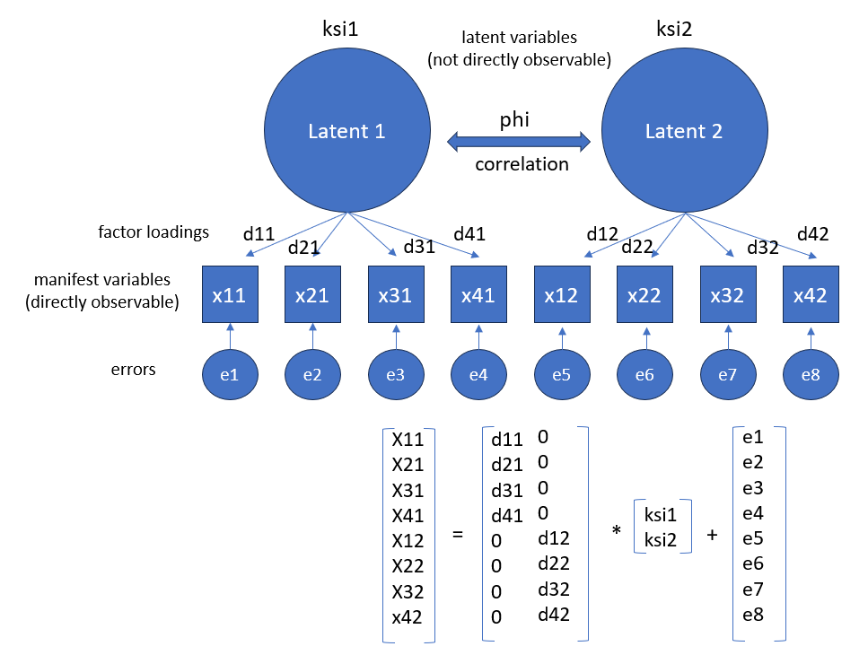
2.3 Types of parameters
- Fixed: are assigned a specific constant value a priori.
- value equals zero: if no causal relationships between certain variables is (theoretically) assumed
- value greater than zero: can be specified, for instance, if the exact effect between two variables is already known in advance
- Constrained: should be estimated in the model, (value should correspond exactly to the value of one or more other parameters).
- If the influence of two variables on a dependent variable is considered to be equal.
- If two parameters are defined as restricted, only one parameter has to be estimated instead of two.
- Free: all other parameters whose values are considered unknown and should be estimated from the empirical data.
3 Model information
3.1 Identification
Step 1: defining a metric for the latent constructs
- The latent variables and error variables to be estimated initially have no metric.
- In order to interpret the variable, a scale must be assigned.
Step 2: identifying the model structure
- A metric for the latent constructs must be defined.
- Check whether there is enough information to estimate the model.
Note: the more complex a model is, the more parameters have to be estimated, and the greater the model’s degrees of freedom must be in order to make the estimation possible.
3.2 Quantity of information
If \(n\) manifest variables are collected, then the empirical variances and covariances of these variables can be calculated:
\[ p = \frac{n(n+1)}{2} \]
\(p\) corresponds to the available “information” for calculating all free parameters of our model. The difference between the available empirical information (\(p\)) and the number of parameters to be estimated (\(q\)) gives the degrees of freedom of the model (\(df_M\)):
\[ df_M = p - q \]
Under- and over-identified models:
- if \(p=q\): the number of model degrees of freedom corresponds to zero (just-identified).
- if \(q>p\): the model is not identified (under-identified).
3.3 Identification methods
Reference Variable (or Marker Method):
- A reference (or marker) variable is chosen, and its factor loading on the latent variable is fixed to 1. This approach requires selecting the best indicator variable to represent the latent construct.
- By fixing this loading to 1, the latent variable is defined in the same metric as the chosen indicator, meaning that the latent variable mirrors the chosen indicator variable except for measurement error.
Fixed Factor Loading (or Variance Standardization Method):
- The variance of the latent variable is fixed (often to 1), and the factor loadings for all measured indicator variables are freely estimated.
- The estimated measurement errors, therefore, reflect any observed variance that is not attributable to the influence of the latent variable.
3.4 Example: under-identified model
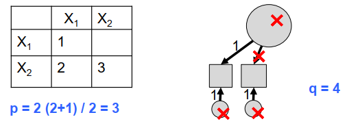
In the following example, the model is under-identified (df < 0): the information available from the empirical data is not sufficient to calculate the parameters.
- 5 total (unique) parameters
- quantity of information to estimate: \(p = \frac{n(n+1)}{2} = 3\)
- 4 free parameters
- degree of freedom: \(p-q = 3-4 = -1\) (under-identified)
3.5 Example: over-identified model
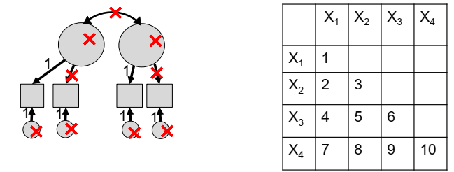
In the model below:
- 11 total (unique) parameters
- quantity of information to estimate: \(p = \frac{4(4+1)}{2} = 10\)
- 9 (11-2) free parameters
- degrees of freedom: \(p-q = 10-9 = 1\) (over-identified)
4 Model quality
4.1 Parameters determination and Fit-indices
Empirical variance-covariance matrix (in short: covariance matrix): calculated with the collected data (= empirical relationships in the data).
Model-theoretical covariance matrix: defined measurement model (= expected relationships in the data).
=> the model-theoretical covariance matrix should resemble the empirical covariance matrix as closely as possible.
Model quality: fit-indices describe how good the model is. Exactly one solution is possible for exactly identified models, several solutions are possible for over-identified models, the best solution must be found.
4.2 Maximum Likelihood and model quality
The parameters can actually be estimated using various functions. The most common method is the so-called Maximum Likelihood (ML) method. The estimated parameter is selected that is most likely to reproduce the observed data.
Once a solution has been found, it must be checked for quality.
- Reliability: Repeated measurements must always produce the same result (items must all show a high loading with the latent construct)
- Validity: the measuring instrument should measure what it is supposed to measure
Multi-stage process:
- Checking at indicator level
- Testing at the construct level
- Examination on model level
4.3 Indicator level examination
We must ensure that only “good” indicators are included in a model:
- sufficiently high correlations between the items (e.g. Cronbach’s Alpha)
- plausibility of the factor loadings
- significance/strength of the factor loadings
- Standardized solution corresponds to factor loadings (as in EFA, values >.5 are desirable)
- Squared factor loadings indicate the percent variance of a variable that is explained by the factor behind it (should reach at least .3)
4.4 Construct level examination
We should assess whether the constructs/factors are reliably and validly measured:
- Factor reliability (should be > .5)
- Average extracted variance of factors (should be > .5)
- Discriminant validity (Fornell/Larcker criterion)
4.5 Model level examination
The examination at model level suggests to check whether the empirical variance-covariance matrix is reproduced as well as possible by the model-theoretical variance-covariance matrix (e.g. Fit-indices, Chi-Square test statistic, RMSEA and SRMR).
- Chi-Square Test (H0: empirical covariance matrix = model-theoretical covariance matrix)
- The smaller the difference between the two matrices, the smaller the chi-square value (the smaller the chi-square, the better).
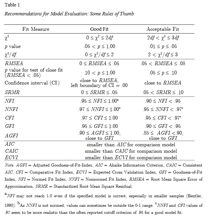
4.6 Guidelines: fit assessement
Table can be found here.
4.7 In case of bad model fit
There are several things we can do if the model fit is too bad:
- adjust model if necessary
- release certain fixed parameters
- find a balance between mathematical fit and theoretical meaning
Comparing different models can be useful when we have competing theoretical models.
Comparison rules:
- lower RMSEA = descriptively better model
- larger CFI = descriptively better model
- smaller AIC = descriptively better model
5 Example in R
5.1 Example: negative campaigning behavior scale
We can use CFA to check a theoretical model for measuring negative campaigning behaviors of politicians using the following variables:
- Criticised particular items on the platform of other parties
- Criticised the records of other parties during the term
- Criticised issues specific to the personal campaign of other candidates
- Criticised personal characteristics and circumstances of other candidates
5.2 Testing the model
# default: marker method by lavaan
syntx <- 'RC1 =~ B9a + B9b + B9c + B9d'
model_cfa <- lavaan::cfa(syntx, data = sel)
summary(model_cfa)
Length Class Mode
1 lavaan S4 lhs op rhs est pvalue
1 RC1 =~ B9a 1.0000000 NA
2 RC1 =~ B9b 1.0751968 0
3 RC1 =~ B9c 1.0159835 0
4 RC1 =~ B9d 0.7518455 0
5 B9a ~~ B9a 0.8377181 0
6 B9b ~~ B9b 0.8805613 0
7 B9c ~~ B9c 0.4378973 0
8 B9d ~~ B9d 0.5384798 0
9 RC1 ~~ RC1 0.7003171 05.3 Visualization
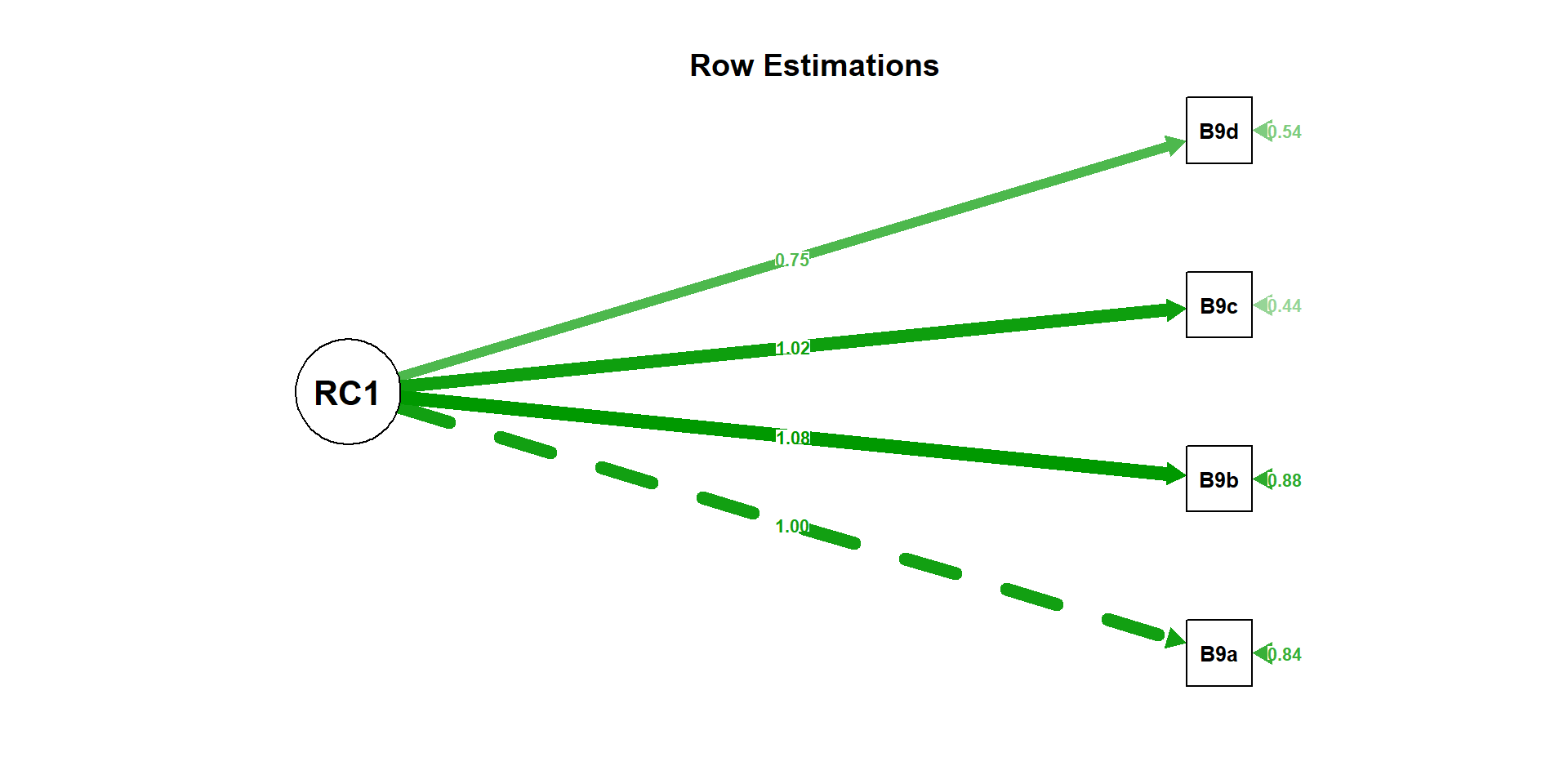
5.4 Model fit
fits <- lavaan::fitMeasures(model_cfa)
data.frame(fits = round(fits[c("ntotal","df",
                               "chisq","pvalue",
                               "rmsea","rmsea.pvalue","srmr")], 2))
fits
ntotal 2074.00
df 2.00
chisq 300.49
pvalue 0.00
rmsea 0.27
rmsea.pvalue 0.00
srmr 0.06
Multivariate statistics