Exploratory factor analysis (EFA) presentation

Learn what EFA is and how to run the analysis in R

1 Exploratory versus confirmatory factor analysis

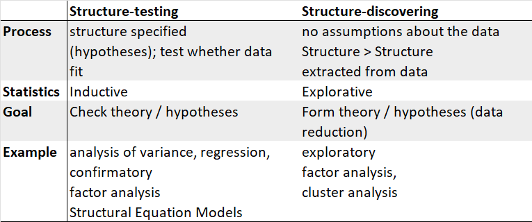
1.1 Conceptual difference

EFA:

In EFA, all measured variables are related to every latent variable.
It is used to reduce data to a smaller set of summary variables and to explore the underlying theoretical structure of the phenomena.
It asks what factors are given in observed data and, thereby, requires interpretation of usefulness of a model.

CFA:

In CFA, researchers can specify the number of factors required in the data and which measured variable is related to which latent variable.
It asks how well a proposed model fits a given data.
It is useful to compare models (and data).

1.2 Differences in both approaches

2 How EFA works

2.1 Prerequisites for dimensionality reduction

There are two main prerequisites:

Condition: There are several interval-scaled characteristics (items).
Rule of thumb: At least 50 people and 3x more people as variables (ideally: 5x more people as variables!).

Dimensionality reduction transforms a data set from a high-dimensional space into a low-dimensional space.

It can be a good choice when you suspect there are too many variables which can be a problem because it is difficult to understand (or visualize) data in higher dimensions.

2.2 Potential consequence of having a multitude of predictors

Possible harm to a model: in linear regression, the number of predictors should be less than the number of data points used to fit the model.
Multicollinearity: between-predictor correlations can negatively impact the mathematical operations used to estimate a model.
Theoretical violations: predictors may be measuring the same latent effect(s), and thus such predictors will be highly correlated.

2.3 Dimensionality reduction methods

There are different ways of combining variables:

linear: Principal component analysis (PCA), Factor analysis (FA), Multiple correspondence analysis (MCA), Linear discriminant analysis (LDA) or Singular value decomposition (SVD)
non-linear: Kernel PCA, t-distributed Stochastic Neighbor Embedding (t-SNE) or Multidimensional scaling (MDS)

Alternatively, we can keep the most important features: Random forests, Forward or Backward selection, among others.

2.4 EFA: general procedure and guidelines

Procedure:

Setup and evaluate data set
Choose number of factors to extract
Extract (and rotate) factors
Evaluate what you have and possibly repeat 2 & 3
Interpret and write-up results

Guidelines:

It is better to select only the variables of interest from the data set.
As factor analysis (and PCA) does not play well with missing data, it is better to remove cases that have missing data.
Remember that factor analysis is designed for continuous data, although it is possible to include categorical data in a factor analysis.

2.5 Suitability of the data

Only relevant items may be included in the factor analysis. For instance, items must correlate significantly.

Here, Bartlett Test is useful to assess the hypothesis that the sample came from a population in which the variables are uncorrelated:

H0: The variables are uncorrelated in the population.
H1: The variables are correlated in the population.

Kaiser-Meyer-Olkin (KMO) criterion and Measure of Sampling Adequacy (MSA) further test to what extent the variance of one variable is explained by the other variables. This indicates whether a data set is suitable for a factor analysis:

value range 0-1
values from .8 desirable
values below .5 unacceptable

3 What factors are

3.1 Spatial representation

In EFA, each variable cannot be fully explained by a linear combination of p factors:

\[ Z_{ij} = f_{i1}a_{1j} + f_{i2}a_{2j} + ... + f_{ip}a_{pj} + e_j\]

This approach should be used when trying to identify latent variables that are crucial to answering the items.

The correlation coefficient between item and factor is the factor loading (\(a_{jn}\)).

Fundamental theorem: every observed value of a variable \(x_j\) can be described as a linear combination of several (hypothetical) factors (\(f_{jn}\)).

3.2 Coefficient of determination

To extract the factors, we can z-standardize all variables (mean=0, standard deviation=1).

To measure the explanation of the variance of a variable, the coefficient of determination represents the square of the factor loading (see \(R^2\) in the linear regression).

The first factor is the z-standardized variable for which the sum of the determination coefficients is maximum.

3.3 Strategies to extract the relevant number of factors

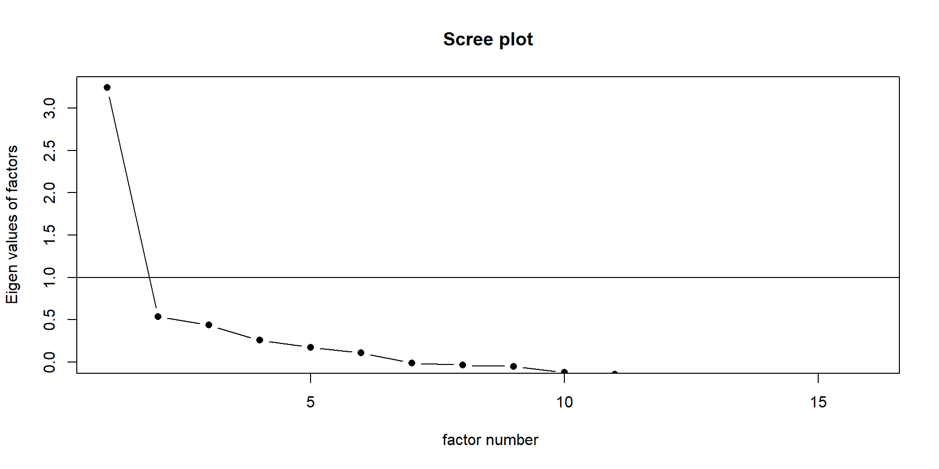
Kaiser criterion: significant factor explains more variance than any of the original variables and this criterion is fulfilled from an eigenvalue of 1 onwards
Scree plot: eigenvalues are plotted in the graphic and the factors that lie above a “threshold” are extracted
Content plausibility: so many factors are accepted that a plausible interpretation results
A priori criterion: it is theoretically determined in advance how many factors there should be

4 Factor rotation

4.1 Types of rotation

By rotation one obtains simple structure, the factor interpretation is relieved.

There are different types of rotation:

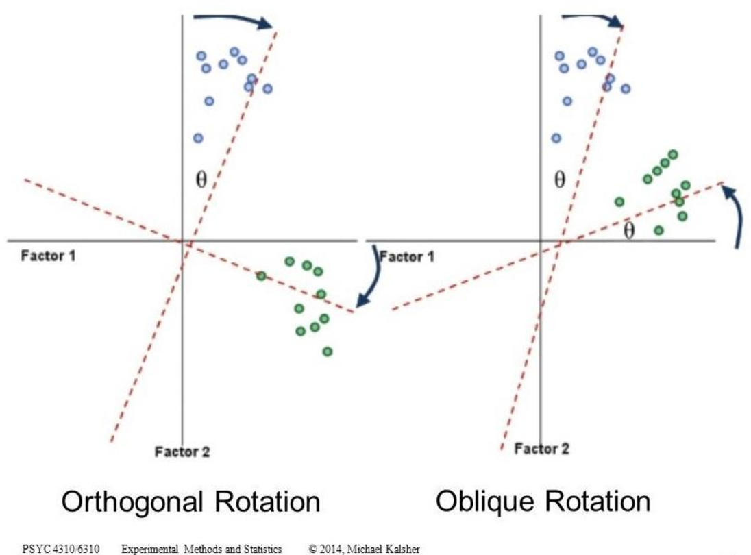
Orthogonal: the factor axes remain at right angles, so that they are uncorrelated
Oblique: the factor axes do not remain at right angles, so that they are correlated
Combination (first right angles and then oblique)

4.2 Which rotation is better?

Which form of factor rotation is chosen in a specific case often depends on the theory behind it.

Orthogonal rotations:

are easier to interpret because the factors are uncorrelated.
are usually appropriate for pure dimension reduction.

Oblique rotations:

appear to make more sense if highly correlated factors are assumed in the data.
do not assume that the various factors are independent and, therefore, uncorrelated.

Practical guideline: start with the assumption that the factors are non-independent (oblique rotation method). If the correlations are fairly low (r<|0.30|), then you could justify the assumption that the factors are independent (orthogonal) and should not be correlated.

4.3 Rotation options

Oblique rotation options:

Promax rotation is popular for its ability to handle large datasets efficiently. The approach also tends to result in greater correlation values between factors.
Oblimin rotation is somewhat less efficient with large datasets, but can produce a simpler factor structure.

Orthogonal rotation options:

Varimax rotation is optimized to reduce cross loadings and to minimize smaller loading values, making factor models clearer.
Quartimax rotation works to reduce the number of variables needed to explain a factor, making interpretation easier.
Equamax rotation offers a compromise between varimax and quartimax.

5 Interpreting and naming the factors

5.1 Factor loadings

Factor interpretation is based on the factor loadings. Loadings from .5 are usually interpreted. Ideally, variables load exactly high on one factor and low on another.

For factor naming, variables with higher loadings should be given more consideration.

A negative charge does not mean that the item does not belong to the factor. However, the sign must be taken into account in the interpretation.

Possible problems:

Loading several variables on several factors poses interpretation difficulties
Negative factor, or one-item factor

5.2 Validation & crossloadings

Validation and internal validity:

You need to assess whether all variables load onto the factors sufficiently. If not: try another method of factor extraction and/or a different number of factors.
It is also important to check that all factors have at least 3 or more variables loading onto them. If not: decrease the number of factors.
Values of Cronbach’s alpha will look a lot like positive correlation values, varying between zero and 1.0. If you see values greater than 1.0, you may have some collinearity issue.

Crossloadings:

Crossloadings (variables that load onto more than one factor) should be unavoidable.
Each factor should be interpretable: variables that load onto each factor have at least a fairly clear theme (based on the variable definitions).

6 Quiz

6.1 Can I answer these questions?

function quizInput({ questions, options}) {
  let answers = questions.map(() => null);
  let root = htl.html`<div
      style="
        display: grid;
        grid-template-columns: 10% 10% 70% 10%;"
    >
      ${options.map(
        (opt) => htl.html`<div style="font-weight: bold">${opt}</div>`
      )}
      <div style="font-weight: bold">Statements</div>
      <div style="font-weight: bold"></div>
      ${Array.from(questions.entries(), ([i, [question, correct]]) =>
        quizInputRow({
          question,
          options,
          correct,
          onChange: (newAnswer) => {
            answers[i] = newAnswer;
            root.value = answers;
            root.dispatchEvent(new CustomEvent("input"));
          }
        })
      )}
    </div>`;
  root.value = answers;
  return root;
}

function quizInputRow({
  question,
  options,
  correct,
  onChange = () => {}
}) {
  let root = htl.html`<div>`;

  function setAnswer(answer, initial = false) {
    morph(
      root,
      htl.html`<div style="display: contents"> 
      <form style="display: contents">
        ${options.map(
          (opt) =>
            htl.html`<label>&emsp;</label> 
            <input  
              name=${question} &emsp;
              type="radio"
              value="${opt}"
              checked=${opt === answer}
              onChange=${() => setAnswer(opt)}
            >
            </input>`
        )}
      </form>
      <div>${question}</div>
      <div> &emsp; ${
       answer === null ? "" : answer === correct ? "🟢" : "🔴"
      }</div>
    </div>`
    );

    root.value = answer;
    if (!initial) {
      root.dispatchEvent(new CustomEvent("input"));
      onChange(answer);
    }
  }

  setAnswer(null, true);
  return root;
}

morph = require("https://bundle.run/nanomorph@5.4.2")

True or false?

MC_1_1 = [
    ["The KMO (Kaiser-Meyer-Olkin criterion) describes the proportion of the variance of an item that is explained by all factors", "false"],
    ["The KMO indicates whether the data are suitable for factor analysis", "true"],
    ["In EFA, each item can initially be fully explained by a linear combination of all factors", "false"],
    ["For factor analyses, the sample size should be at least N=20", "false"]
]

viewof answers_1_1 = quizInput({
  questions: MC_1_1,
  options: ["true", "false"]
})

Punkte_1_1 = {
const Sum = 
    (answers_1_1[0] == MC_1_1[0][1])*1 + 
    (answers_1_1[1] == MC_1_1[1][1])*1 + 
    (answers_1_1[2] == MC_1_1[2][1])*1 + 
    (answers_1_1[3] == MC_1_1[3][1])*1 

var Punkte_1_1 = Sum - 2
if (Punkte_1_1 < 1) {Punkte_1_1 = 0}
return(Punkte_1_1)
}

Score:

7 Example in R

7.1 Data selection

In the following example, we will look for the best categorization of political candidates’ campaign tools (e.g., door-knocking, mailing lists, Facebook posts, etc). This could then lead to create scores for the each of the candidates’ communication patterns.

We first select the necessary variables and make sure that they are in a numeric format.

library(foreign)
db <- read.spss(file=paste0(getwd(),
                "/data/1186_Selects2019_CandidateSurvey_Data_v1.1.0.sav"), 
                use.value.labels = T, 
                to.data.frame = T)
sel <- db |>
  dplyr::select("B4a","B4b","B4c","B4d","B4e","B4f","B4g","B4h","B4i","B4j",
                "B4k","B4l","B4m","B4n","B4o","B4p") |>
  stats::na.omit() 
for(i in 1:ncol(sel)){sel[,i] <- as.numeric(sel[,i])-1}

7.2 Correlation analysis

If some variables are too highly correlated (r>0.90), then it is better to select one variable from each pair to omit from the data set:

M <- cor(sel)
round(M, 1)

    B4a B4b B4c B4d B4e B4f B4g B4h B4i B4j B4k B4l B4m B4n B4o B4p
B4a 1.0 0.4 0.3 0.2 0.2 0.2 0.2 0.1 0.2 0.3 0.2 0.1 0.2 0.1 0.0 0.2
B4b 0.4 1.0 0.2 0.1 0.3 0.2 0.2 0.1 0.1 0.2 0.1 0.1 0.2 0.1 0.0 0.1
B4c 0.3 0.2 1.0 0.1 0.2 0.1 0.2 0.1 0.1 0.1 0.1 0.1 0.2 0.1 0.0 0.1
B4d 0.2 0.1 0.1 1.0 0.3 0.3 0.3 0.2 0.3 0.2 0.3 0.2 0.2 0.1 0.1 0.1
B4e 0.2 0.3 0.2 0.3 1.0 0.3 0.3 0.1 0.2 0.2 0.2 0.1 0.2 0.2 0.1 0.1
B4f 0.2 0.2 0.1 0.3 0.3 1.0 0.5 0.1 0.3 0.3 0.3 0.2 0.3 0.1 0.2 0.2
B4g 0.2 0.2 0.2 0.3 0.3 0.5 1.0 0.1 0.3 0.3 0.3 0.1 0.3 0.1 0.1 0.2
B4h 0.1 0.1 0.1 0.2 0.1 0.1 0.1 1.0 0.2 0.2 0.3 0.4 0.1 0.3 0.1 0.1
B4i 0.2 0.1 0.1 0.3 0.2 0.3 0.3 0.2 1.0 0.4 0.4 0.2 0.2 0.1 0.2 0.2
B4j 0.3 0.2 0.1 0.2 0.2 0.3 0.3 0.2 0.4 1.0 0.3 0.2 0.3 0.2 0.1 0.2
B4k 0.2 0.1 0.1 0.3 0.2 0.3 0.3 0.3 0.4 0.3 1.0 0.3 0.3 0.1 0.2 0.3
B4l 0.1 0.1 0.1 0.2 0.1 0.2 0.1 0.4 0.2 0.2 0.3 1.0 0.1 0.2 0.2 0.2
B4m 0.2 0.2 0.2 0.2 0.2 0.3 0.3 0.1 0.2 0.3 0.3 0.1 1.0 0.3 0.2 0.3
B4n 0.1 0.1 0.1 0.1 0.2 0.1 0.1 0.3 0.1 0.2 0.1 0.2 0.3 1.0 0.1 0.1
B4o 0.0 0.0 0.0 0.1 0.1 0.2 0.1 0.1 0.2 0.1 0.2 0.2 0.2 0.1 1.0 0.2
B4p 0.2 0.1 0.1 0.1 0.1 0.2 0.2 0.1 0.2 0.2 0.3 0.2 0.3 0.1 0.2 1.0

7.3 KMO test and Bartlett’s test for sphericity

We can also run the KMO test which serves as a criterion overall and for each variable in a correlation matrix. The following values are generally acceptable: >0.7

psych::KMO(sel)

Kaiser-Meyer-Olkin factor adequacy
Call: psych::KMO(r = sel)
Overall MSA =  0.85
MSA for each item = 
 B4a  B4b  B4c  B4d  B4e  B4f  B4g  B4h  B4i  B4j  B4k  B4l  B4m  B4n  B4o  B4p 
0.83 0.76 0.86 0.88 0.84 0.86 0.86 0.77 0.87 0.87 0.87 0.81 0.87 0.76 0.89 0.87

The null hypothesis for Bartlett’s test is that the correlation matrix equals the identity matrix (rule out that the variables in the data set are essentially uncorrelated). If you fail to reject the null for this test, it suggests that there is nothing in there for you to factor (the variables are all essentially different from one another).

bartlett = psych::cortest.bartlett(sel)
print(paste0("Chi-2: ", round(bartlett[["chisq"]],2), 
             "; p-value: ", bartlett[["p.value"]]))

[1] "Chi-2: 5346.19; p-value: 0"

7.4 Latent structure & Eigenvalue

We are seeking latent structure within a set of data, and we will only be interested in factors that explain a substantial proportion of variation within the data.

The eigenvalue method (Kaiser’s rule) is telling us that 4 factors may be best.

ev <- eigen(cor(sel)) 
print(ev$values)

 [1] 3.9952969 1.3683021 1.2531488 1.0666162 0.9749318 0.8854319 0.8582437
 [8] 0.8378168 0.7351154 0.7056058 0.6258888 0.5984852 0.5563688 0.5371627
[15] 0.5244517 0.4771334

The scree plot is putting us somewhere between 2 and 4 factors:

psych::scree(sel, pc=FALSE)

7.5 Oblique rotation: oblimin

fit <- psych::fa(sel, nfactors=4, rotate="oblimin")
summary(fit)


Factor analysis with Call: psych::fa(r = sel, nfactors = 4, rotate = "oblimin")

Test of the hypothesis that 4 factors are sufficient.
The degrees of freedom for the model is 62  and the objective function was  0.19 
The number of observations was  1973  with Chi Square =  381.58  with prob <  1.6e-47 

The root mean square of the residuals (RMSA) is  0.03 
The df corrected root mean square of the residuals is  0.04 

Tucker Lewis Index of factoring reliability =  0.881
RMSEA index =  0.051  and the 10 % confidence intervals are  0.046 0.056
BIC =  -88.83
 With factor correlations of 
     MR1  MR2  MR3  MR4
MR1 1.00 0.33 0.41 0.51
MR2 0.33 1.00 0.21 0.31
MR3 0.41 0.21 1.00 0.22
MR4 0.51 0.31 0.22 1.00

print(fit$loadings, digits=2, cutoff=0.3, sort=T)


Loadings:
    MR1   MR2   MR3   MR4  
B4d  0.52                  
B4f  0.57                  
B4g  0.63                  
B4i  0.50                  
B4h        0.72            
B4a              0.51      
B4b              0.64      
B4m                    0.50
B4c              0.32      
B4e  0.43                  
B4j  0.31                  
B4k  0.32              0.35
B4l        0.49            
B4n                        
B4o                        
B4p                    0.47

                MR1  MR2  MR3  MR4
SS loadings    1.66 0.96 0.94 0.80
Proportion Var 0.10 0.06 0.06 0.05
Cumulative Var 0.10 0.16 0.22 0.27

7.6 Orthogonal rotation: varimax

fit2 <- psych::fa(sel, nfactors=4, rotate="varimax")
summary(fit2)


Factor analysis with Call: psych::fa(r = sel, nfactors = 4, rotate = "varimax")

Test of the hypothesis that 4 factors are sufficient.
The degrees of freedom for the model is 62  and the objective function was  0.19 
The number of observations was  1973  with Chi Square =  381.58  with prob <  1.6e-47 

The root mean square of the residuals (RMSA) is  0.03 
The df corrected root mean square of the residuals is  0.04 

Tucker Lewis Index of factoring reliability =  0.881
RMSEA index =  0.051  and the 10 % confidence intervals are  0.046 0.056
BIC =  -88.83

print(fit2$loadings, digits=2, cutoff=0.3, sort=T)


Loadings:
    MR1   MR4   MR3   MR2  
B4f  0.54  0.30            
B4g  0.58                  
B4m        0.53            
B4a              0.53      
B4b              0.63      
B4h                    0.69
B4c              0.34      
B4d  0.47                  
B4e  0.41        0.33      
B4i  0.48                  
B4j  0.35                  
B4k  0.37  0.47            
B4l                    0.49
B4n                        
B4o                        
B4p        0.47            

                MR1  MR4  MR3  MR2
SS loadings    1.65 1.21 1.16 1.03
Proportion Var 0.10 0.08 0.07 0.06
Cumulative Var 0.10 0.18 0.25 0.32

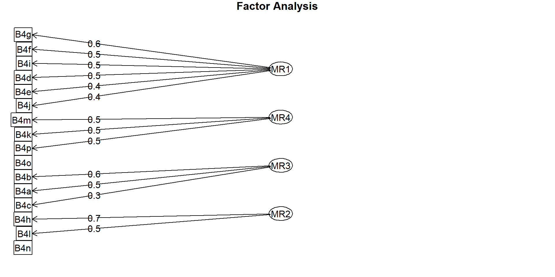
7.7 Visualization and cluster naming

loads <- fit2$loadings
psych::fa.diagram(loads)

Cluster 1: a: Door-knocking; b: Distributing campaign material; c: Calling up voters

Cluster 2: d: Visiting businesses and organisations; e: Meetings with party elites/members/groups f: Media activities ; g: Public speeches and rallies; i: Personal ads

Cluster 3: k: Personal website or blog; m: Facebook; p: Twitter

Cluster 4: h: Direct mailing; l: Mailing list

7.8 Chronbach’s alpha

We can check the internal validity of the factors:

f1 <- sel[,c("B4a","B4b","B4c")]
f2 <- sel[,c("B4d","B4e","B4f","B4g","B4i")]
f3 <- sel[,c("B4k","B4m","B4p")]
f4 <- sel[,c("B4h","B4l")] # should be combined or removed

The raw-alpha value for the entire factor tells us how consistent the variables are within the factor:

alpha = psych::alpha(f1, check.keys=T) # check.keys=T allows to reverse negative loadings
print(alpha$total[1:2])

 raw_alpha std.alpha
 0.5409754 0.5371888

For one specific factor:

psych::alpha(f1, check.keys=TRUE)$total[1]

 raw_alpha
 0.5409754

The next thing to consider is the way alpha would change if each of the variables were removed.