setwd("./data/SHP/")
ff <- list.files()
pp <- data.frame()
for(i in 1:length(ff))
{
  p <- foreign::read.spss(ff[i], to.data.frame = T)
  sel <- p[,grepl("P.*P01|P.*P07|P.*P08|P.*P09",colnames(p))]
  sel <- as.data.frame(sel)
  if(ncol(sel)<4){next}
  sel <- cbind(p$IDPERS,sel)
  colnames(sel) <- c("IDPERS",
                     paste0("polint_",substr(ff[i],1,5)),
                     paste0("boycott_",substr(ff[i],1,5)),
                     paste0("strike_",substr(ff[i],1,5)),
                     paste0("demo_",substr(ff[i],1,5)))

  if(i==1){pp <- cbind(p$SEX00,p$AGE00,sel)}
  if(i>1){pp <- merge(pp,sel,by="IDPERS",all.x=T)}
}
for(i in 4:ncol(pp)){pp[,i] <- as.numeric(pp[,i])}
# save(pp, file="SHP_PoliticalEngagment.RData")Latent Growth Curve Modelling (LGM) presentation
Learn what LGM are and how to run the analysis in R
Latent Growth Modelling (LGM)
LGM allows us to investigate longitudinal trends or group differences in measurement (also called growth trajectories).
For example, suppose we want to model the political (or their political political engagement) polarization of panel participants over time.
Recap: lavaan syntax
- ~ predict, used for regression of observed outcome to observed predictors
- =~ indicator, used for latent variable to observed indicator in factor analysis measurement models
- ~~ covariance
- ~1 intercept or mean (e.g., q01 ~ 1 estimates the mean of variable q01)
- 1* fixes parameter or loading to one
- NA* frees parameter or loading (useful to override default marker method)
- a* labels the parameter ‘a’, used for model constraints
- c(a,b)* specifically for multigroup models, see note below
Understanding the concept of LGM
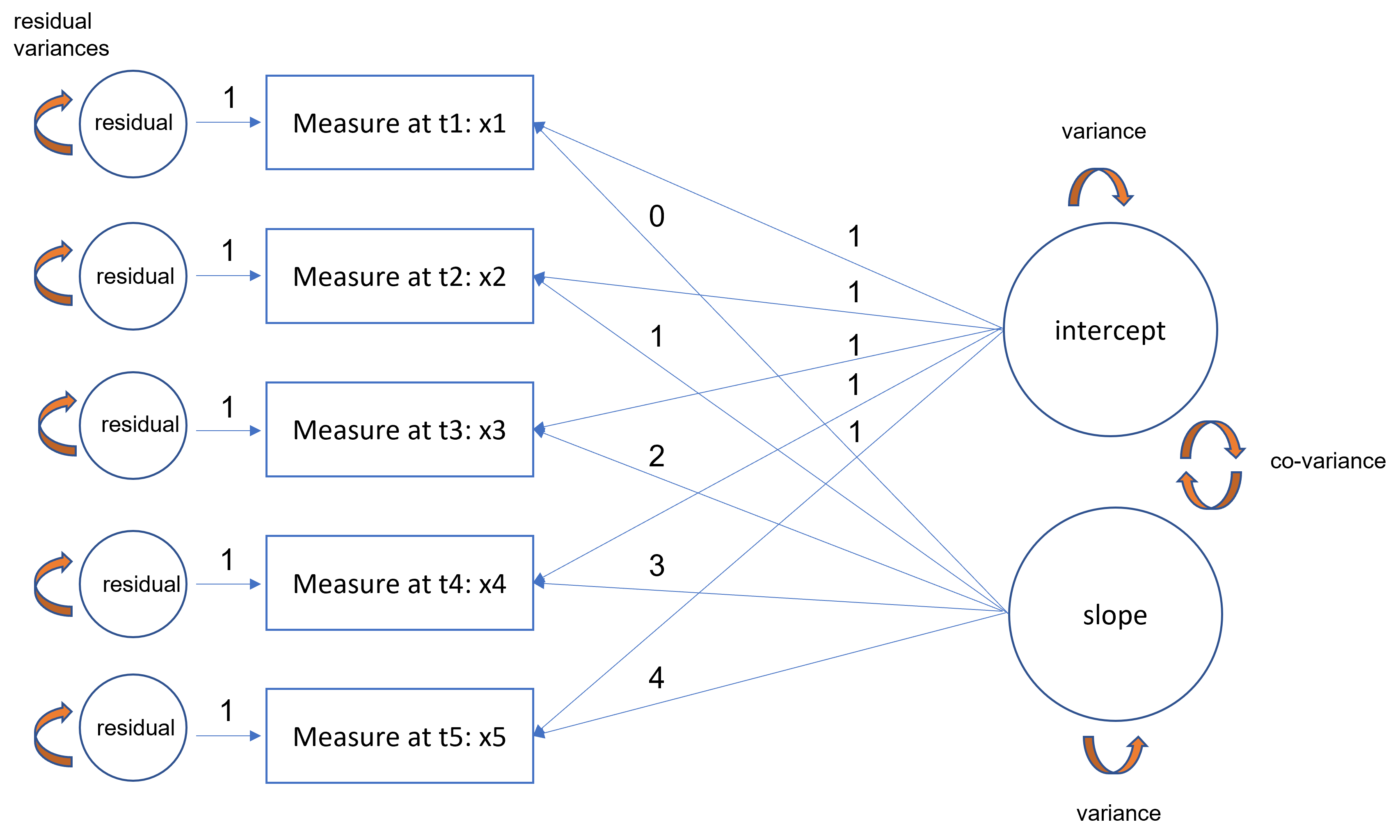
LGM can be considered as an extension of the CFA model where the intercepts are freely estimated.
Most commonly:
- the loadings for the intercept factor are all fixed to 1
- the loadings for the linear slope factor can be any ordered progression
- the first loading of the slope factor is fixed to 0
- the progression proceeds ordinally in increments of 1
- a one-unit increase in time is interpreted as an increase in the predicted outcome for a fixed time interval increase
Difference with CFA
Unlike traditional CFA models where the interpretation focuses on the loadings, the loadings are fixed in GLM which implies that the focus is on the latent intercept and linear slope factors.
For GLM, the dataset should be structured in wide format: each column represents the outcome (or dependent variable) at a specific timepoint. An assumption is that each observation or row must be independent of another. However, columns indicating outcomes are time dependent.
Diagram example

Equations
Each time point is defined for a person as follows:
\[ x_{it} = \tau_{i} + \xi_{1} + (t)\xi_{2} + \delta_{it} \]
where the observed intercepts are constrained to be zero (\(\tau_{i}=0\)).
The (symmetric) variance covariance matrix of the latent intercept and slope is defined as:
\[ \Phi = \begin{bmatrix} \phi_{11}\\ \phi_{21} & \phi_{22} \end{bmatrix} \]
where \(\phi_{11}\) is the variance of the latent intercept, \(\phi_{22}\) is the variance of the latent slope and \(\phi{21}\) is the covariance of the intercept and slope. The population parameters correspond to the latent intercept and linear slope means.
Ordinal versus measured time in an LGM
The fixed loadings for the slope factor can be defined in different way depending on how time is modeled.
- For instance, it can be assumed that time is measured ordinally (in increments of year or semester), regardless of the actual measured time (the loadings will be 0,1,2,3,…).
- In other situations, it may be more beneficial to use measured time, such as for a study design where assessments are implemented at baseline, 3-, 6-, 9-, and 12-month follow-up (the loadings will be fixed at 0, 3, 6, 9 and 12), thus corresponding to the actual time of assessment.
Equivalence of LGM and MLM
The format of the dataset for LGM should be in long format with repeated observations of time spanning multiple rows of data for every subject.
This suggests that the LGM model is equivalent to an MLM with time nested within individuals with the following specifications:
- inclusion of a fixed effect of time at Level 1
- addition of a random intercept clustered by student and a random slope of time (indicated as time|student with the lmer syntax)
\[ y_{ij} = \beta_{0j} + \beta_{1j}*TIME_{ij} + r_{ij} \] \[ \beta_{0j} = \gamma_{00} + u_{0j} \] \[ \beta_{1j} = \gamma_{10} + u_{1j} \]
Unconstrained residual variances
The important difference between the default LGM and MLM is that the residual variances of the LGM are unconstrained across time points but are constrained to be the same across time in a HLM by default.
Note: to constrain the residual variances in an LGM, we can use the a* notation in the lavaan syntax. In that case, the interpretation of the output is exactly the same for the LGM as it is for the HLM.
Adding a predictor to the LGM
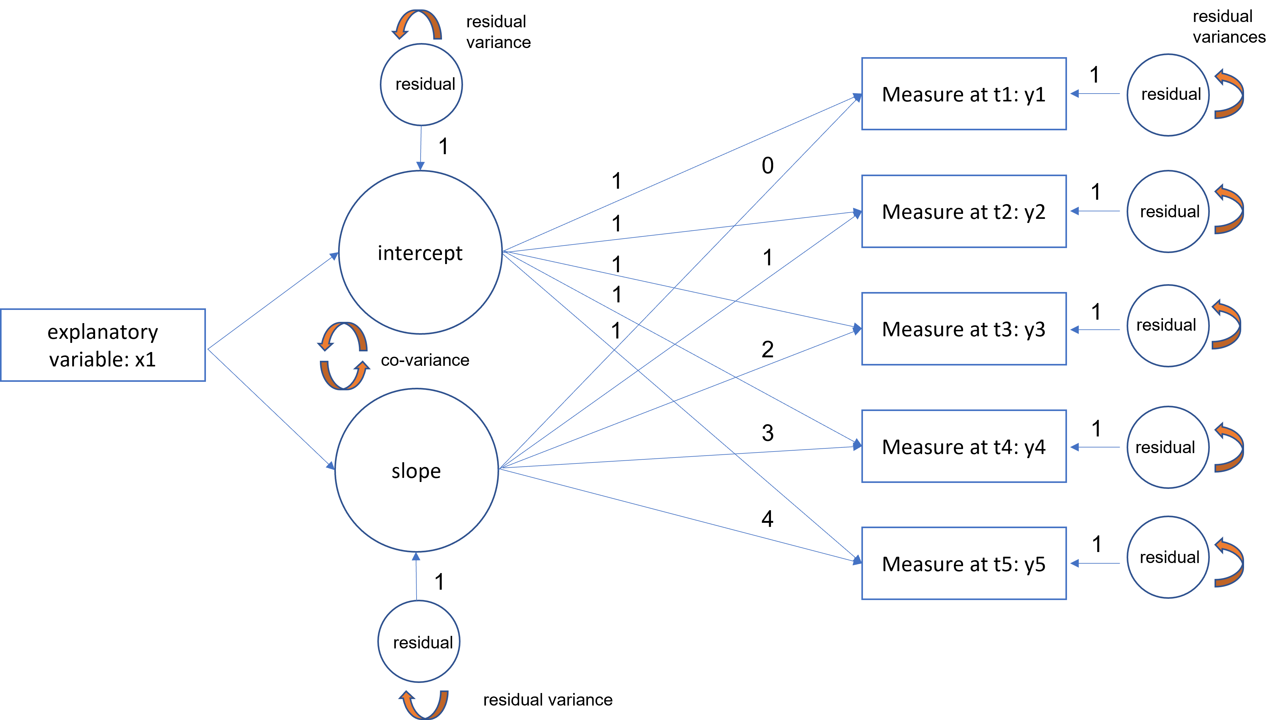
Now, we would like to find out what are potential predictors of this linear trajectory.
For example, if the trajectory of political involvement increases over time, how does political affiliation predict this trend? Are there ideological differences in either the starting political involvement (intercept factor) or the growth trajectory (slope factor)?
We would have the following specifications:
- latent factors now have a predictor
- latent intercept and slope factors become endogenous (y-side variables)
- there is a residual term which was not in the exogenous model (replace the variance of factor with the residual factor term)
- additional of an exogenous predictor (x1)
Example

Example in R: political engagement
First, we need to prepare the data in a long format so that each columns represents a time observation for each respondent:
LGM with lavaan
Then, we can specify an LGM in lavaan using the growth() function, which is a wrapper function for the lavaan() function that automatically specifies fixed and free parameters for the latent growth model.
load(file=paste0(getwd(),"/data/SHP/SHP_PoliticalEngagment.RData"))
sel <- pp[complete.cases(pp),]
sel$engagement00 <- sel$boycott_SHP00+sel$strike_SHP00+sel$demo_SHP00
sel$engagement01 <- sel$boycott_SHP01+sel$strike_SHP01+sel$demo_SHP01
sel$engagement02 <- sel$boycott_SHP02+sel$strike_SHP02+sel$demo_SHP02
sel$engagement03 <- sel$boycott_SHP03+sel$strike_SHP03+sel$demo_SHP03
sel$engagement04 <- sel$boycott_SHP04+sel$strike_SHP04+sel$demo_SHP04
sel$engagement05 <- sel$boycott_SHP05+sel$strike_SHP05+sel$demo_SHP05
# specify the model for the first 5 years
library(lavaan)
m1 <-   'i =~ 1*engagement00 + 1*engagement01 + 1*engagement02 + 1*engagement03 + 1*engagement04 + 1*engagement05
         s =~ 0*engagement00 + 1*engagement01 + 2*engagement02 + 3*engagement03 + 4*engagement04 + 5*engagement05'
lgm_m1 <- growth(m1, data=sel)
t <- summary(lgm_m1)
Outputs
            lhs op          rhs         est       pvalue
13 engagement00 ~~ engagement00 25.06681149 0.000000e+00
14 engagement01 ~~ engagement01 27.91081732 0.000000e+00
15 engagement02 ~~ engagement02 23.46821938 0.000000e+00
16 engagement03 ~~ engagement03 21.71316657 0.000000e+00
17 engagement04 ~~ engagement04 19.66577747 0.000000e+00
18 engagement05 ~~ engagement05 16.90900447 0.000000e+00
19            i ~~            i 69.92693007 0.000000e+00
20            s ~~            s  0.52386351 3.819167e-14
21            i ~~            s -0.10004141 7.523647e-01
28            i ~1              15.26025297 0.000000e+00
29            s ~1               0.05377592 8.992581e-02
Looking at the output above, the predicted political engagement in the first year (i.e., 2000) is 15.260 and for every sequential year is expected to go up by 0.054 points.
The parameters \(\phi_{11}\)=69.927 and \(\phi_{22}\)=0.524 represents the variances of the intercept and slope across respondents.
Interpretatin
Taking the square root of the variance gives us the standard deviation and assuming normality, a 95% plausible value ranges for mean engagement across respondents is \(15.260\pm{1.96\sqrt{69.927}}\) and for the slope is \(0.054\pm{1.96\sqrt{0.524}}\).
Finally, the estimated covariance \(\phi_{22}=-0.100\) which implies that there is a negative relationship between the intercept and slope: the higher the starting value of engagement, the weaker the increase in engagement over time.
GLM comparison with MLM
To compare the results of GLM with MLM, we need to prepare a long format data structure:
long = sel[,c("IDPERS","engagement00","engagement01","engagement02","engagement03","engagement04","engagement05" )]
long <- data.table::melt(data.table::setDT(long), id.vars = c("IDPERS"), variable.name = "engagement")
long$time = NA
long$time[long$engagement=="engagement00"] <- 0
long$time[long$engagement=="engagement01"] <- 1
long$time[long$engagement=="engagement02"] <- 2
long$time[long$engagement=="engagement03"] <- 3
long$time[long$engagement=="engagement04"] <- 4
long$time[long$engagement=="engagement05"] <- 5
long$engagement = NULL
colnames(long)[2]="engagement"
MLM output
lmer_fit1 <- lme4::lmer(engagement ~ time + (time|IDPERS), data=long)
stargazer::stargazer(lmer_fit1, type="text", single.row = T)
===============================================
                        Dependent variable:
                    ---------------------------
                            engagement
-----------------------------------------------
time                      0.072** (0.032)
Constant                 15.215*** (0.218)
-----------------------------------------------
Observations                  10,428
Log Likelihood              -33,944.770
Akaike Inf. Crit.           67,901.530
Bayesian Inf. Crit.         67,945.050
===============================================
Note:               *p<0.1; **p<0.05; ***p<0.01
To obtain the covariance, we can use the function VarCorr() which takes in an lmer object:
Constraining residual variances of LGM
To find equivalent results in lavaan, we need to constrain the residual variances of LGM:
m2 <- 'i =~ 1*engagement00 + 1*engagement01 + 1*engagement02 + 1*engagement03 + 1*engagement04 + 1*engagement05
       s =~ 0*engagement00 + 1*engagement01 + 2*engagement02 + 3*engagement03 + 4*engagement04 + 5*engagement05
       engagement00 ~~ a*engagement00
       engagement01 ~~ a*engagement01
       engagement02 ~~ a*engagement02
       engagement03 ~~ a*engagement03
       engagement04 ~~ a*engagement04
       engagement05 ~~ a*engagement05'
lgm_fit2 <- growth(m2, data=sel)
t <- summary(lgm_fit2)
Outputs
            lhs op          rhs         est       pvalue
13 engagement00 ~~ engagement00 22.61911553 0.000000e+00
14 engagement01 ~~ engagement01 22.61911553 0.000000e+00
15 engagement02 ~~ engagement02 22.61911553 0.000000e+00
16 engagement03 ~~ engagement03 22.61911553 0.000000e+00
17 engagement04 ~~ engagement04 22.61911553 0.000000e+00
18 engagement05 ~~ engagement05 22.61911553 0.000000e+00
19            i ~~            i 70.88447140 0.000000e+00
20            s ~~            s  0.47960373 6.616929e-14
21            i ~~            s -0.24409383 4.267095e-01
28            i ~1              15.21486186 0.000000e+00
29            s ~1               0.07170798 2.472538e-02
We can confirm that the covariance of the intercept and slope is \(\phi_{12}=-0.244\) and \(\theta_{\delta}=22.619\) from lavaan matches the output from lmer, showing the equivalence of the LGM and HLM.
Adding predictors
Recall that we constrain the residual variance of engagement to be the same across timepoints to show equivalency with HLM. In order to specify gender as a predictor of the intercept use syntax i ~ sex and slope use s ~ sex to denote regression:
colnames(sel)[2] <- "gndr"
m3 <-   '
         i =~ 1*engagement00 + 1*engagement01 + 1*engagement02 + 1*engagement03 + 1*engagement04 + 1*engagement05
         s =~ 0*engagement00 + 1*engagement01 + 2*engagement02 + 3*engagement03 + 4*engagement04 + 5*engagement05
         i ~ gndr
         s ~ gndr
         engagement00 ~~ a*engagement00
         engagement01 ~~ a*engagement01
         engagement02 ~~ a*engagement02
         engagement03 ~~ a*engagement03
         engagement04 ~~ a*engagement04
         engagement05 ~~ a*engagement05'
lgm_fit3 <- growth(m3, data=sel)
t <- summary(lgm_fit3)
Outputs
            lhs op          rhs        est       pvalue
13            i  ~         gndr -1.0481912 1.774658e-02
14            s  ~         gndr  0.1373765 3.380286e-02
15 engagement00 ~~ engagement00 22.6191160 0.000000e+00
16 engagement01 ~~ engagement01 22.6191160 0.000000e+00
17 engagement02 ~~ engagement02 22.6191160 0.000000e+00
18 engagement03 ~~ engagement03 22.6191160 0.000000e+00
19 engagement04 ~~ engagement04 22.6191160 0.000000e+00
20 engagement05 ~~ engagement05 22.6191160 0.000000e+00
21            i ~~            i 70.6177876 0.000000e+00
22            s ~~            s  0.4750231 1.001421e-13
23            i ~~            s -0.2091418 4.944161e-01
32            i ~1              16.8764048 0.000000e+00
33            s ~1              -0.1460549 1.740305e-01
Female and male respondents differ in their starting engagement in the first year: females have an estimated -1.048 lower engagement than males (intercept).
Female respondents have a linear growth trajectory that is 0.137 units higher than male respondents across the years (slope).
Adding a time predictor
long <- merge(long,sel[,c("IDPERS","gndr")], by="IDPERS", all.x=T)
lmer_fit2 <- lme4::lmer(engagement ~ time + gndr + time:gndr + (time|IDPERS),data=long)
stargazer::stargazer(lmer_fit2, type="text", single.row = T)
===============================================
                        Dependent variable:
                    ---------------------------
                            engagement
-----------------------------------------------
time                      -0.009 (0.050)
gndrwoman                -1.048** (0.442)
time:gndrwoman            0.137** (0.065)
Constant                 15.828*** (0.338)
-----------------------------------------------
Observations                  10,428
Log Likelihood              -33,942.580
Akaike Inf. Crit.           67,901.170
Bayesian Inf. Crit.         67,959.190
===============================================
Note:               *p<0.1; **p<0.05; ***p<0.01
To obtain the variances and covariances:
       grp        var1 var2       vcov       sdcor
1   IDPERS (Intercept) <NA> 70.7193833  8.40948175
2   IDPERS        time <NA>  0.4770668  0.69070021
3   IDPERS (Intercept) time -0.2134422 -0.03674697
4 Residual        <NA> <NA> 22.6187645  4.75591889
Multivariate statistics