function quizInput({ questions, options}) {
let answers = questions.map(() => null);
let root = htl.html`<div
style="
display: grid;
grid-template-columns: 10% 10% 70% 10%;"
>
${options.map(
(opt) => htl.html`<div style="font-weight: bold">${opt}</div>`
)}
<div style="font-weight: bold">Statements</div>
<div style="font-weight: bold"></div>
${Array.from(questions.entries(), ([i, [question, correct]]) =>
quizInputRow({
question,
options,
correct,
onChange: (newAnswer) => {
answers[i] = newAnswer;
root.value = answers;
root.dispatchEvent(new CustomEvent("input"));
}
})
)}
</div>`;
root.value = answers;
return root;
}
function quizInputRow({
question,
options,
correct,
onChange = () => {}
}) {
let root = htl.html`<div>`;
function setAnswer(answer, initial = false) {
morph(
root,
htl.html`<div style="display: contents">
<form style="display: contents">
${options.map(
(opt) =>
htl.html`<label> </label>
<input
name=${question}  
type="radio"
value="${opt}"
checked=${opt === answer}
onChange=${() => setAnswer(opt)}
>
</input>`
)}
</form>
<div>${question}</div>
<div>   ${
answer === null ? "" : answer === correct ? "🟢" : "🔴"
}</div>
</div>`
);
root.value = answer;
if (!initial) {
root.dispatchEvent(new CustomEvent("input"));
onChange(answer);
}
}
setAnswer(null, true);
return root;
}
morph = require("https://bundle.run/nanomorph@5.4.2")Linear regression presentation
Learn what linear regression is and how to run the analysis in R
1 Linear regression
1.1 Definition and application
- It is an important method as it allows an easy transition to multivariate data analysis.
- It also allows an extension to categorical data analysis, as well as hierarchical models.
In its simplest form, linear regression is a way of predicting value of one variable Y through another known variable X.
It is a hypothetical model which uses the equation of a straight line (linear model) based on the method of least squares which minimize the sum of squared errors (SSE).
What does this mean?
1.2 Basic example
Let’s take a basic example covering the relationship between years of education (X) and income (Y).
Which income can be attained with ten years of education? Answering this question requires finding the best fitting line between the two variables with the formula:
\[\mathbf{\hat{y_i}} = \mathbf{a} + \mathbf{b}\;\mathbf{x_i}\]
- \(\mathbf{\hat{y_i}}\) is the estimated income for an individual,
- \(\mathbf{a}\) is the constant (or intercept: value where education equals 0),
- \(\mathbf{x_i}\) is the value of education for an individual,
- \(\mathbf{b}\) is the effect size of education on income (or slope).
1.3 Equation for the slope
The equation for the slope is represented by dividing the covariance over the variance:
\[\mathbf{b}=\frac{\sum^{}_{}(x-\overline{x})\times(y-\overline{y})}{\sum^{}_{}(x-\overline{x})^2}=\frac{s_{xy}}{s_x^2}\]
1.4 Best fitting line
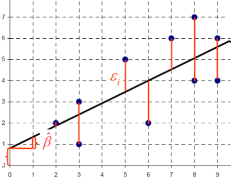
In principle, there are plenty of lines through the data and the line with the lowest SSE (Sum of Squared Errors) represents the line which best fit the data.
In our example, the predicted income deviates from the observed income, because all values are not lying precisely on a line.
Therefore, we need to estimate a regression line where distances (errors) between the predicted and observed values are minimized. The residuals read as follows:
\[\mathbf{\hat{\epsilon}} = \mathbf{y}-\mathbf{\hat{y_i}}=\mathbf{y_i}-\hat{\alpha}-\hat{\beta}\mathbf{x_i}\]
Up to here, we are able to interpret the slope coefficient, which gives us the direction of the effect (+ or -) and the extent to which Y changes if X increases by 1.
However, we also need to assess the statistical significance of the effect.
2 Variance
2.1 Confidence interval
The slope coefficient represents the point estimator (sample) for the “true” population value (\(\beta\)).
The standard error provides us with a measure for the variability (dispersion) of \(\mathbf{b}\) and, thereby, the confidence intervals to test significance of the effect.
The null hypothesis states that there is no relation between X and Y.
2.2 Total variation
How much variance is there on the Y?
We are interested in the overall variation. Therefore, without knowing X, the mean of Y is the best estimate for all Y values.
This is also called the “baseline model” and the resulting error is called total variation:
\(TSS = \sum{(Y_i - \overline{Y})^2}\)
However, knowing X, the regression line is a better estimate for Y. The resulting error is the residual variation (“residuals”):
\(SSE = \sum{(Y_i - \hat{Y}_i)^2}\)
Therefore, the explained variation in the regression model is:
\(MSS = \sum{(\hat{Y}_i - \overline{Y})^2}\)
2.3 Representation
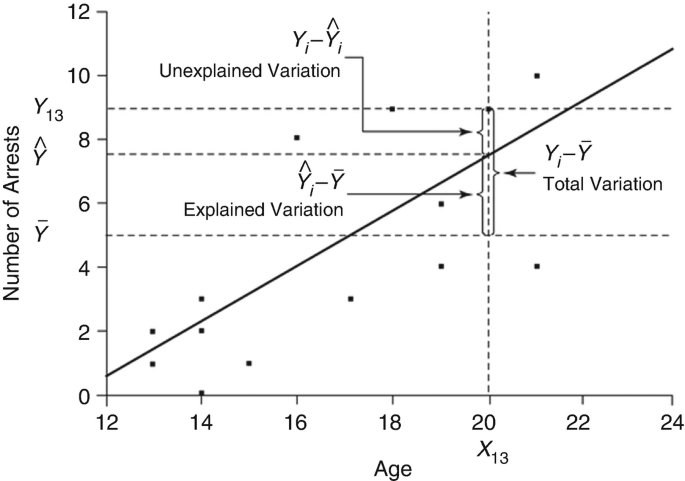
The original figure can be found here.
3 Multivariate model
3.1 Additional explanatory factors
In real world, the relations between two variables are often influenced by “third variables”.
In this case, the bivariate association is not informative if not controlling for the disturbing influence of a third, fourth, fifth, etc. variable (with different measurement levels).
Multivariate regression takes the influence of other variables on the relation between two variables into account. Therefore, it is powerful to detect spurious- and suppressor effects, indirect effects, and interaction effects.
3.2 Net influence
The goal is to estimate the “net” influence of several independent variables:
\[\mathbf{\hat{y}} = \mathbf{a} + \mathbf{b_1}\;\mathbf{x_1} + \mathbf{b_2}\;\mathbf{x_2} + \mathbf{b_k}\;\mathbf{x_k}\]
In multivariate models, the \(b\) coefficient represents the “raw” regression coefficient.
3.3 Comparison of coefficients
The comparison of \(b\) coefficients is not meaningful if the variables are measured in different units (e.g. working time in hours & family size in number of individuals).
A possible solution is the standardization of the variables (mean=0 & standard deviation=1) in view of assessing which independent variable has greater effect on Y (relative contribution).
The standardized \(b\) (written by convention \(\beta\)) are often referred as the beta coefficients.
The interpretation of the \(\beta\) coefficient indicates by how many standard deviations Y varies when X varies by one standard deviation.
4 Explained proportion of the variance
4.1 \(R^2\)
\(R^2\) provides us with a measure of accuracy of the regression model, that is how well does the regression line approximate the real data points.
It represents the share of explained variance (how much variation in Y is explained through X) and varies between 0 and +1.
\(R^2\) tends to increase as we increase the number of variables in the model.
\(R^2\) does not tell us whether the independent variables are true cause of changes in Y (no causality), whether omitted-variable bias exists (third variable problem), whether the correct regression was used, and whether appropriate independent variables have been chosen.
In research, our focus is often only one part of a complex story.
4.2 \(R^2\) explained
\[R^2=\frac{TSS-SSE}{TSS}=\frac{MSS}{TSS}\]
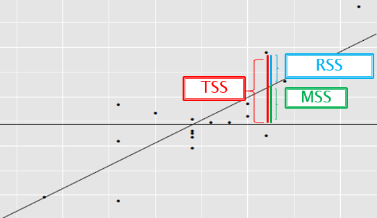
- TSS: total sum of squares
- SSE (or RSS): sum of squares of residuals
- MSS: model sum of squares
4.3 Relationship between \(r\) and \(R^2\)
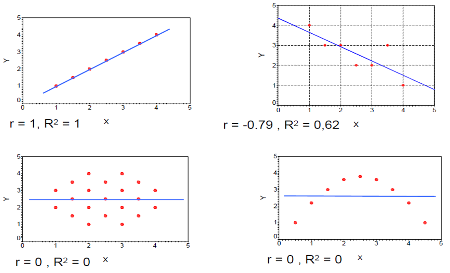
If X and Y are two metric variables, \(R^2\) is a measure of a linear relation between X and Y, while \(r\) (Pearson correlation) is the empirical correlation between X and Y.
Importantly, in bivariate regression, \(R^2 = r_{xy}^2\) (where \(r\) is a standardized regression coefficient).
In multiple regression, \(r\) represents the correlation between the observed \(y\) values and the predicted \(\hat{y}\) values.
5 Model quality
5.1 F-test for the regression model
F-test is a global check of the regression model. It tests the hypothesis whether in the population there is a connection between the Y and the X:
- H0: no connection (or \(R^2\) = 0)
- H1: there is a connection (or \(R^2\) not equal 0)
5.2 Standard estimation error
The standard estimation error characterizes the spread of the y-values around the regression line and is therefore a quality measure for the accuracy of the regression prediction:
\[ s_e = \sqrt{\frac{\sum{(Y_i - \hat{Y}_i)^2}}{n-k-1}} \]
The standard error of estimation comes from the fact that:
- Part of the estimation error can be attributed to chance (e.g. “human randomness”)
- Part is determined by predictors that are not included in the model
- Part of the estimation error arises from measurement errors
5.3 Overfitting
The regression equation is always exactly identified if the number of observations is only one higher than the number of independent variables (if: n-1 = k).
There are only sufficient “degrees of freedom” if there are more measuring points (observations) than variables.
Only if the deviations are small, then we are talking about a high quality of fit of the regression calculation.
5.4 Potential issues with overfitting
Specific sample features only apply to one sample, not to the total population and not to other samples either. They should not be allowed to contribute to model quality.
As a consequence, the estimate always tends to be too high. That means:
- The estimated Y values and the empirical Y values correlate (probably) stronger than in reality
- The residuals are smaller than they should actually be (according to the conditions in the population)
- The explained variance is consequently greater than it should be
5.5 Shrinkage
The determination coefficient often turns out to be smaller with a new sample.
This phenomenon/principle is called shrinkage.
Therefore, a corrected \(R^2\) (adjusted \(R^2\)) takes this into account by reducing the simple \(R^2\) by a correction value that is larger: the larger the number of predictors and the smaller the number of cases.
Whereas the \(R^2\) increases with each added predictor, the corrected \(R^2\) decreases as more (irrelevant or non-informative) predictors are added. Adjusted \(R^2\) adjusts for model complexity and can move in either direction depending on the predictor’s usefulness.
5.6 Statistical significance
A t-test is used to determine whether the regression coefficients deviate significantly from zero (H0). To calculate the t-value per coefficient, the standard error (\(S_b\)) of each coefficient is also necessary.
The \(S_b\) characterizes the spread of the regression coefficients around the population parameter and is therefore a quality measure for the accuracy of the parameter estimation.
The larger the standard error, the smaller the empirical t-value and the less likely it is that the H0 will be rejected.
5.7 Nota bene
The significance of the effect is based on the ratio between a coefficient and its standard error.
This is the empirical value of the t-test (\(t=b/S_b\)), which is compared with a critical value (c.v.=1.96).
The null hypothesis (H0) is accepted if the critical value is < 1.96. The confidence interval should not contain 0.
6 Dummy variables
6.1 Reference category
Categorical independent variables are problematic because the numeric codes assigned to their categories are arbitrary (when the code changes, the estimate changes).
A solution suggests associating a binary dummy variable with each modality (coded 0 and 1).
A categorical variable with c modalities is replaced by c-1 dummies.
The omitted modality serves as a reference category.
The choice of the reference category is made on the basis of empirical considerations (e.g., modality with the largest number of cases or modality that makes sense from a theoretical point of view).
The coefficients \(b\) are interpreted with respect to the reference category.
7 Postulates and assumptions
7.1 No miss-specification
A regression model should contain exactly those independent variables that are relevant for the dependent variable, no more and no less. Bivariate regression models, for example, are always miss-specified.
The risk with having too few variables is underfitting, thus leading to too high regression coefficients insufficient explanations.
The risk with too many/irrelevant variables is overfitting, thus leading relevant significances to disappear and/or random significance to arise.
To conduct linear regression, we must have sufficient degrees of freedom. In general, this corresponds to at least 10 (or 20) times more cases than variables.
7.2 No multicollinearity
There must be an independence of the independent variables, that is an absence of multicollinearity between the independent variables.
Regression coefficients can be biased if there is a strong correlation between two independent variables.
Multicollinearity is not a severe violation of linear regression (only in extreme cases).
In the presence of multicollinearity, the estimates are still consistent, but there is an increase in standard errors (estimates are less precise).
The problem occurs when researchers include many highly correlated variables (e.g., age and birth year).
Therefore, there should be a theory-driven, careful, and intelligent variable selection.
7.3 Multicollinearity detection
Collinearity statistics include the Tolerance which varies from 0 to 1 and must not be <0.4.
The VIF (variance inflation factor) measure can also be used which varies from 1 to \(\infty\) and must not be >2.5.
If there is multicollinearity, there are basically two solutions:
- either eliminating one (or more) problematic variables,
- or merging the problematic variables (e.g., in a scale).
The Tolerance and VIF are calculated as follows:
- Tolerance = \(1-R^2\)
- VIF = \(1/(1-R^2)\)
7.4 Normality
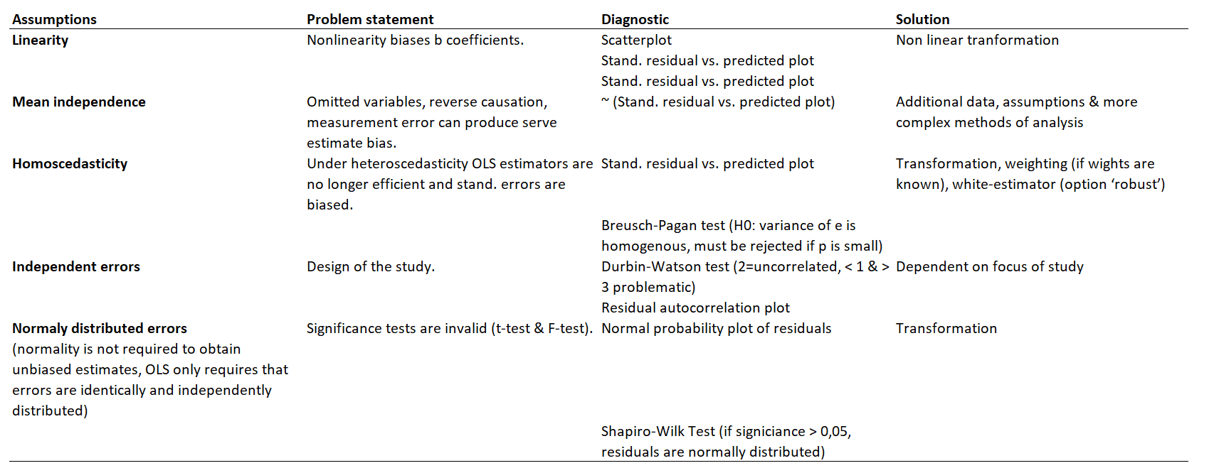
Linear regression only works well for (almost) normally distributed variables. When normality does not apply, we might think about transforming the variables (e.g., log, powers, etc.).
7.5 Homoscedasticity
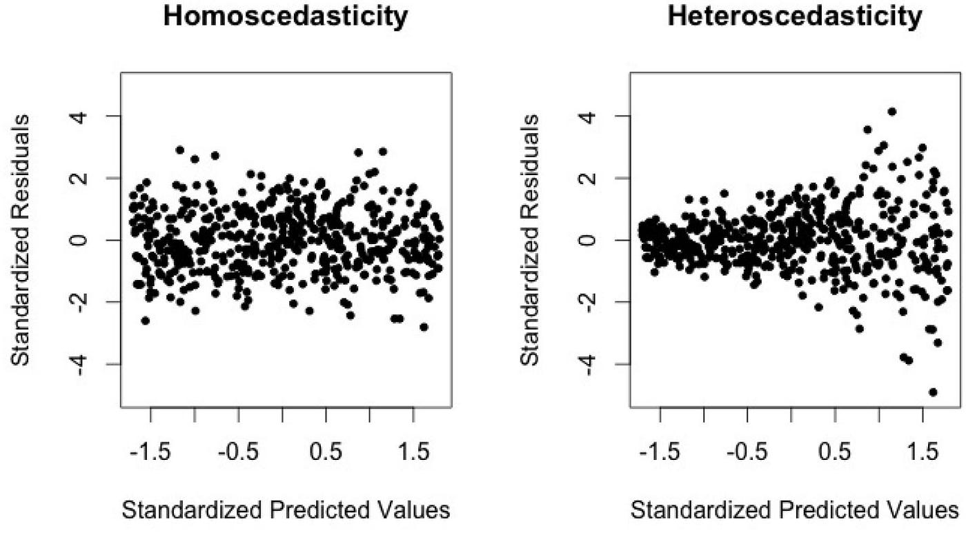
Linear regression also requires homoscedasticity, that is the fact that the variance of the error terms is constant for all values of the independent variables.
Heteroscedasticity is present when there is a relationship between the estimated y-values and the residuals of the observation values.
This can be verified by a visual inspection - no pattern should be discernible.
7.6 No auto-correlation
Furthermore, the error terms must be distributed according to a normal law and should be zero on average.
There must also be an independence of error terms (to be checked when we have time series).
8 Normal distribution of the residuals
The residuals must be normally distributed. For instance, the deviations between estimated and observed values should be zero or close to zero in most cases.
Risks of non-normal residuals result in biased results, thus the significance tests are biased. As a reminder:
- for every empirical value Y there is an estimated value Y and a residual
- the larger the residual for an estimate, the worse the regression estimate for this estimate
- the larger the residuals are overall, the larger the standard estimation error (“mean” of the squared residuals), and the poorer the overall goodness of fit of the regression estimate
8.1 Autocorrelation of the residuals (independent errors)
The non-independence of the residuals occurs when sampling is not independent of one another, i.e. systematically related (time series data, periodic surveys). In these cases, the risks are:
- Bias in the standard error of the regression coefficients
- Bias in the confidence interval for the regression coefficients
We can verify this using the Durbin-Watson statistics.
8.2 Recap

8.3 Outliers
The impact of an observation is depending on two factors.
First, the discrepancy (or outlierness) which assesses observations with large residual (observations whose Y value is unusual given its values on X).
Second, the leverage which assesses observations with extreme value on X with the general rule:
\[lev>(2k+2)/n\]
(with k independent variables in the model).
- A “high leverage” outlier impacts the model fit, may not have big residuals, and can increase \(R^2\).
- A “low leverage” outlier has a lower impact on the model fit, has usually a big residual, inflates standard errors, and decreases \(R^2\).
8.4 Strategies to detect outliers
There are several strategies to identify outliers:
- conducting frequency analysis one variable,
- using the scatterplots for two variables,
- looking at the \(n\) highest and lowest values,
- investigating the residuals (through partial residual plots or added value plots)
We can also rely on influential measures, such as:
- Cook’s Distance with the general rule: \(d>4/(n-k-1)\)
- \(df_{beta}\) with the general rule: \(2/\sqrt{n}\)
8.5 Nota bene on outliers
There might be cases where we want to keep outliers.
This may include cases where we have meaningful cluster (e.g., important subgroup in the data) or cases where outliers might reflect a “real” pattern in the data.
In these cases, it is important to present the results both with and without outliers.
8.6 Diagnostics
9 Interaction effects
9.1 Purpose of interactions
Interaction effects enable us to model non-additive effects. In additive models, the effects of independent variables are the same for the complete sample (e.g., effect of education on income is the same for women and men).
But, theoretically, effect should differ for different groups (e.g., women and men).
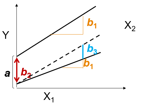
Interaction effects suggest that the strength of the association between \(x_1\) and\(y\) is dependent on the level of a third variable \(x_2\):
\[y=a+b_1x_1+b_2x_2+b_3(x_1 \times x_2)+\epsilon\]
9.2 Interaction between interval variables
For instance, we might be interested in the effect of age (\(x_1\)) on income (\(y\)) depending on years of schooling (\(x_2\)).
In this case, the interpretation of the main effect of \(x_1\) is the effect of \(x_1\) if \(x_2\) equals 0 (and conversely for \(x_2\)).
The interpretation of the interaction effect is done by calculating the effect of \(x_1\) on \(y\) for different levels of \(x_2\) (and conversely for \(x_2\)).
9.3 Interpreting interaction between interval variables
Note that the interpretation of interval variables might be problematic if the zero value is not meaningful (e.g., age=0).
A better interpretation of the main effects can be obtained by centering the variables (through subtracting the mean score from each data-point).
In this case, the interpretation of the intercept (\(a\)) also changes and represents the predicted value of \(y\) if \(x\) is the average.
9.4 Interaction between dummy and interval variables
For instance, we might be interested in how the association between years of education (\(x_1\)) and income (\(y\)) varies by gender (\(x_2\), where 1=women and 0=men).
In this case, the slope (\(b\)) and intercept (\(a\)) of the regression of \(x_1\) on \(y\) are dependent on specific values of \(x_2\). Therefore, for each individual value of \(x_2\) (e.g., 0/1) there is a regression line.
The general interpretation rules suggest that the main effect of \(x_1\) represents the effect of \(x_1\) if \(x_2\) equals 0 (and conversely for \(x_2\)).
Thus, the interaction effect indicates how much the effect of \(x_1\) changes with an unit change in \(x_2\) (and conversely for \(x_2\)).
9.5 Visualization
9.6 Interaction between ordinal and nominal variables
For instance, we might be interested in how the association between the fact of having a child (\(x_1\), where 1=having (at least) a child and 0=no child) and income (\(y\)) varies by gender (\(x_2\), where 1=women and 0=men).
10 Quiz
10.1 Can I answer these questions?
True or false?
MC_1_1 = [
    ["The slope in a linear regression equation represents the effect size of the independent variable on the dependent variable", "true"],
    ["The Sum of Squared Errors (SSE) in a regression model measures the total variance in the dependent variable", "false"],
    ["A high leverage outlier in regression analysis can increase the R-squared value and impact the model fit", "true"],
    ["Interaction effects in regression models account for non-additive effects, meaning the effect of one variable can depend on the level of another variable", "true"]
]

viewof answers_1_1 = quizInput({
  questions: MC_1_1,
  options: ["true", "false"]
})

Punkte_1_1 = {
const Sum =
    (answers_1_1[0] == MC_1_1[0][1])*1 +
    (answers_1_1[1] == MC_1_1[1][1])*1 +
    (answers_1_1[2] == MC_1_1[2][1])*1 +
    (answers_1_1[3] == MC_1_1[3][1])*1

var Punkte_1_1 = Sum - 2
if (Punkte_1_1 < 1) {Punkte_1_1 = 0}
return(Punkte_1_1)
}
Score:
11 Empirical example in R
11.1 Example
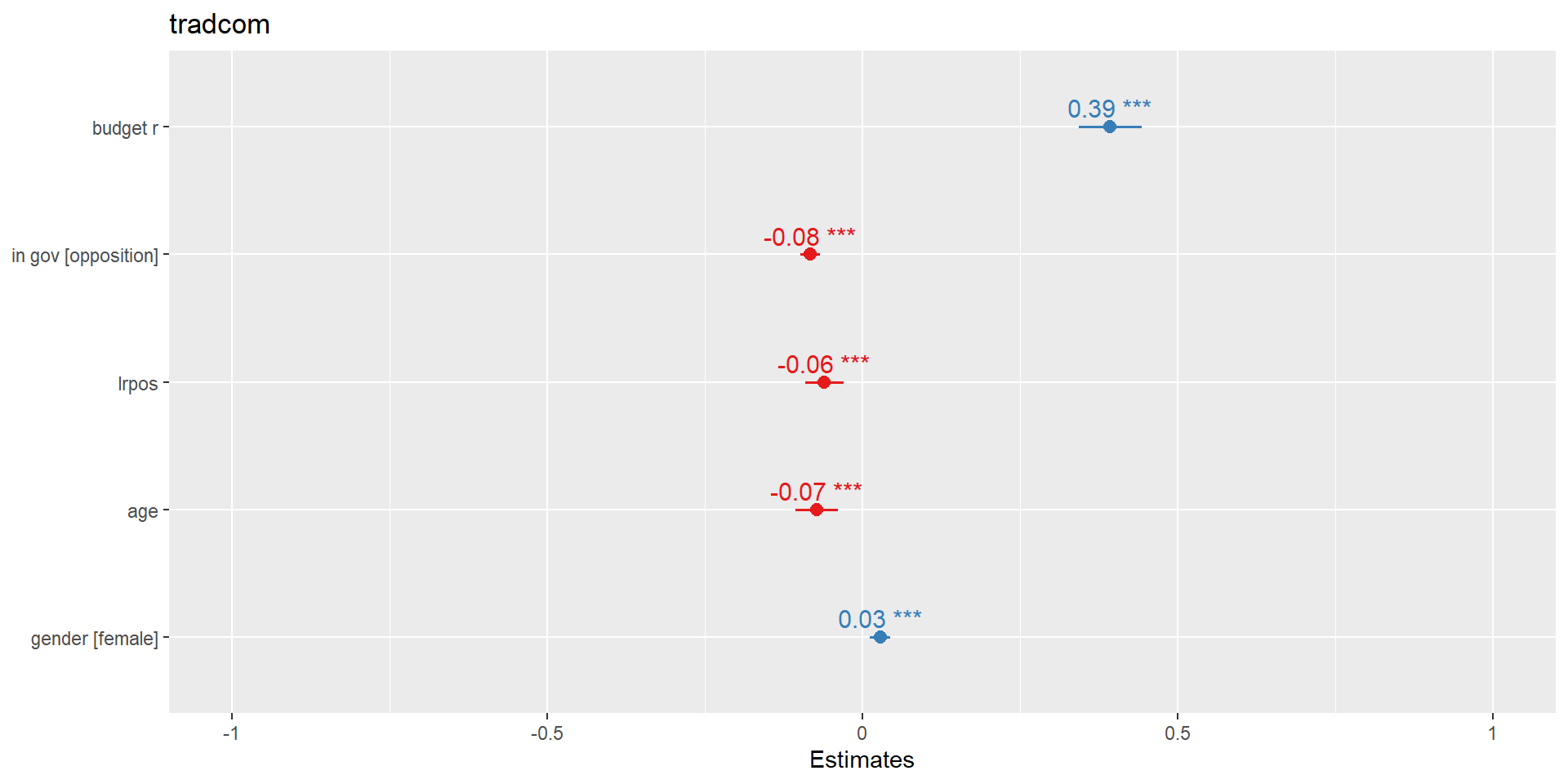
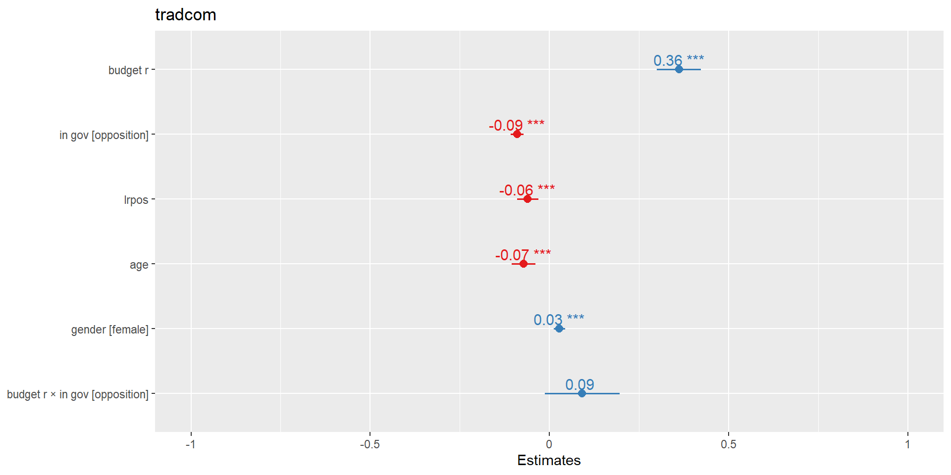
We would like to (partially) explain the reliance on traditional campaign activities by looking at the impact of:
- campaign budget
- party membership in government vs. to a party in opposition (binary variable)
- the interaction term (budget X membership in government)
In addition, we control for the effect of positioning on the left-right axis, as well as age and gender of the candidates.
11.2 Data preparation
We first load the dataset and select the needed variables:
library(foreign)
library(dplyr)
db <- read.spss(file=paste0(getwd(),
                  "/data/1186_Selects2019_CandidateSurvey_Data_v1.1.0.sav"),
                use.value.labels = F,
                to.data.frame = T)
sel <- db |>
  dplyr::select(B12,T9a,C5a,E2a,E1,B4a,B4b,B4c,B4d,B4e,B4g,B4i,B4j) |>
  stats::na.omit() |>
  dplyr::rename("budget"="B12",
                "party_list"="T9a",
                "lrpos"="C5a",
                "age"="E2a",
                "gender"="E1")
11.3 Recoding: variables levels
Them we make sure that the variables have the correct measurement level, and we create a score of traditional media use:
sel <- sel |>
  plyr::mutate(budget=as.numeric(budget)) |>
  plyr::mutate(party_list=as.factor(party_list)) |>
  plyr::mutate(lrpos=as.numeric(lrpos)) |>
  plyr::mutate(B4a=as.numeric(B4a)) |>
  plyr::mutate(B4b=as.numeric(B4b)) |>
  plyr::mutate(B4c=as.numeric(B4c)) |>
  plyr::mutate(B4d=as.numeric(B4d)) |>
  plyr::mutate(B4e=as.numeric(B4e)) |>
  plyr::mutate(B4g=as.numeric(B4g)) |>
  plyr::mutate(B4i=as.numeric(B4i)) |>
  plyr::mutate(B4j=as.numeric(B4j)) |>
  plyr::mutate(tradcom = (B4a+B4b+B4c+B4d+B4e+B4g+B4i+B4j)/8)
11.4 Recoding: gender
We can recode gender so that male are the reference category:
11.5 Recoding: opposition vs government parties
Next, we can create a variable stating whether each candidate is part of a government or opposition party:
# create variable: in government versus opposition
sel$in_gov <- ifelse(sel$party_list==2 | # CVP/PDC
                       sel$party_list==1 | # FDP/PLR
                       sel$party_list==3 | # SP/PS
                       sel$party_list==4, # SVP/UDC
                     "party in gov","opposition")
sel$in_gov <- as.factor(sel$in_gov)
table(sel$in_gov)/nrow(sel)
  opposition party in gov
    0.483165     0.516835
11.6 Recoding budget
We can verify whether there are extreme observations on the budget variable (here: if budget > 50,000).
   Min. 1st Qu.  Median    Mean 3rd Qu.    Max.
0 120 1000 8124 5000 1500000 We can also rescale the budget by multiplying it by 1000 so that we observe the effect of a change of CHF 1000.- units:
Nota bene: We can also apply a log tranformation to make the distribution more normally distributed.
11.7 Scaling the variables
In order to make the coefficient comparable, it is necessary to scale all the numeric variables between 0 and 1:
# keep only valid observations
sel <- sel |>
  dplyr::select(tradcom, budget_r,in_gov, lrpos, age, gender)
sel <- sel[complete.cases(sel),]
# rescale variables
scale_values <- function(x){(x-min(x))/(max(x)-min(x))}
sel$lrpos <- scale_values(sel$lrpos)
sel$age <- scale_values(sel$age)
sel$budget_r <- scale_values(sel$budget_r)
sel$tradcom <- scale_values(sel$tradcom)
Nota bene: the categorical variables should be dummy variables (0/1). In R, the relevel() function can also be used to define the reference category.
11.8 Linear regression
Let’s conduct the linear regression using the lm() funciton:
11.8 Linear regression
11.9 Get \(R^2\)
R-squared is the percentage of the dependent variable variation that a linear model explains. In our model, it explains:
Interpretation: R-squared ranges between 0% and 100%: the larger the R2, the better the regression model fits the observations.
11.10 Diagnostics
- Before assessing numeric measures of goodness-of-fit, like R-squared, you should typically evaluate the residual plots
- Residual plots can expose a biased model (problematic patterns in the residuals)
- If your model is biased, you can neither trust the results of the regression nor the R-squared
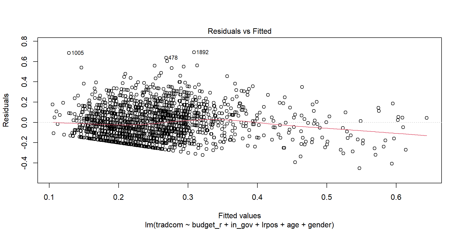
11.11 Linearity
Ideally, this plot would not have a pattern where the red line (lowes smoother) is approximately horizontal at zero.
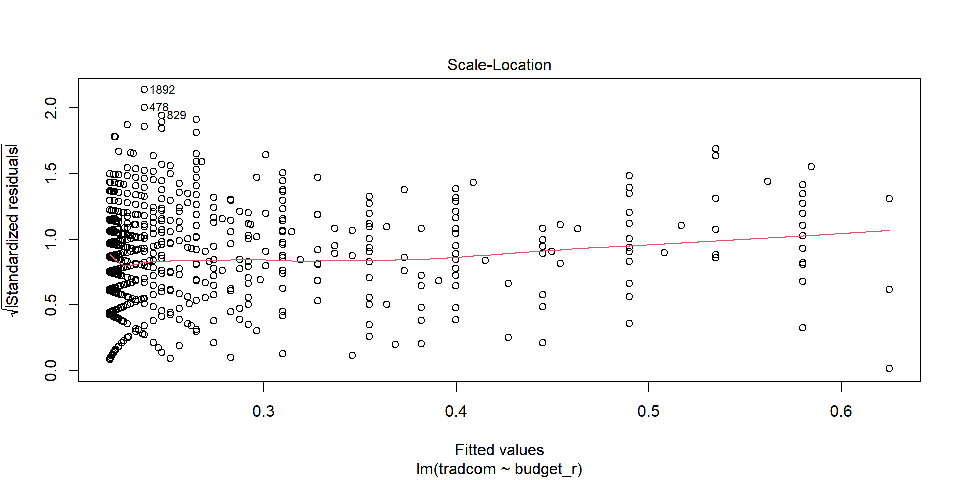
11.12 Homosced.
This plot shows if residuals are spread equally along the ranges of predictors. It is good if you see a horizontal line with equally spread points.
11.13 Errors
Using the Durbin-Watson test, the null hypothesis states that the errors are not auto-correlated with themselves. Thus, if p-value > 0.05, we would fail to reject the null hypothesis.
 lag Autocorrelation D-W Statistic p-value
   1       0.1271508      1.744856       0
 Alternative hypothesis: rho != 0
If there is no autocorrelation, the Durbin-Watson statistic should be between 1.5 and 2.5 and the p-value will be above 0.05.
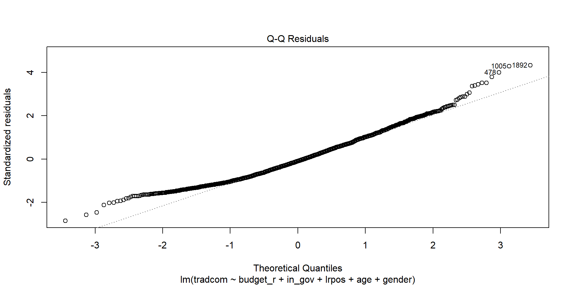
11.14 Residuals
The normal probability plot of residuals should approximately follow a straight line.
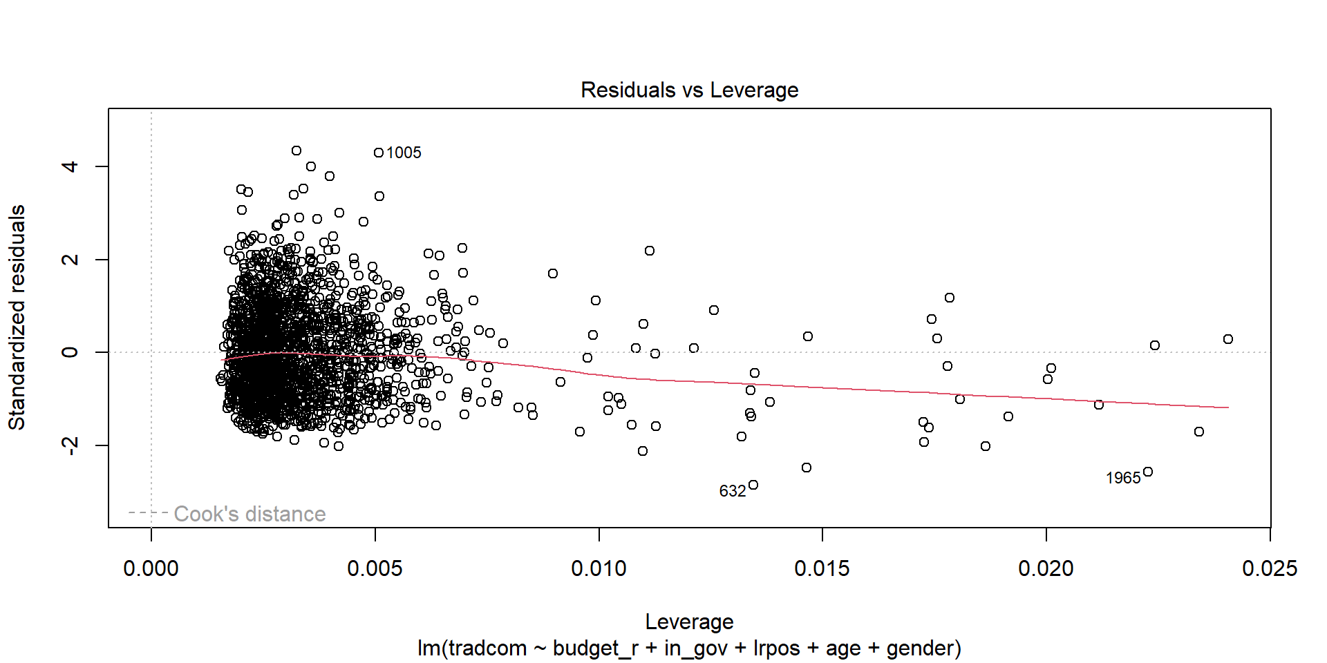
11.15 Outliers
A value of this statistic >2(p+1)/n indicates an observation with high leverage, where p is the number of predictors and n is the number of observations (in our case: 2*(5+1)/1709=0.007)
11.16 Note on outliers
To extract outliers, you might want to flag observations whose leverage score is more than three times greater than the mean leverage value as a high leverage point.
model_data <- broom::augment(model)
high_lev <- dplyr::filter(model_data,.hat>3*mean(model_data$.hat))
high_lev
# A tibble: 35 × 13
.rownames tradcom budget_r in_gov lrpos age gender .fitted .resid .hat
<chr> <dbl> <dbl> <fct> <dbl> <dbl> <fct> <dbl> <dbl> <dbl>
1 177 0.812 0.667 opposi… 0.3 0.343 female 0.464 0.348 0.0111
2 297 0.375 0.711 opposi… 0.1 0.614 male 0.446 -0.0713 0.0135
3 342 0.438 0.667 opposi… 0.4 0.443 male 0.423 0.0144 0.0108
4 392 0.281 0.889 opposi… 0.6 0.414 male 0.500 -0.219 0.0191
5 444 0.438 0.667 opposi… 0.5 0.5 female 0.441 -0.00327 0.0113
6 513 0.656 0.889 party … 0.5 0.529 female 0.609 0.0473 0.0176
7 545 0.188 0.667 opposi… 0.5 0.529 female 0.439 -0.251 0.0113
8 566 0.406 0.889 opposi… 0 0.143 female 0.584 -0.178 0.0212
9 632 0.0938 0.778 party … 0.6 0.314 male 0.547 -0.453 0.0134
10 683 0.438 0.889 party … 0.6 0.229 male 0.597 -0.159 0.0181
# ℹ 25 more rows
# ℹ 3 more variables: .sigma <dbl>, .cooksd <dbl>, .std.resid <dbl>11.17 Multicollinearity
There are several steps to test for multicollinearity issues: theory, correlation, VIF (and tolerance)
             tradcom   budget_r       lrpos         age
tradcom   1.00000000 0.35131999 -0.04394531 -0.06747831
budget_r  0.35131999 1.00000000  0.04767377  0.12998466
lrpos    -0.04394531 0.04767377  1.00000000  0.09041532
age -0.06747831 0.12998466 0.09041532 1.00000000 Variables Tolerance VIF
1 budget_r 0.9689332 1.032063
2 in_govopposition 0.9275798 1.078074
3 lrpos 0.8925535 1.120381
4 age 0.9708446 1.030031
5 genderfemale 0.9541766 1.04802411.18 Interaction effects
Now, we want to know whether the effect of budget is different for candidates from a government or opposition party.
Therefore, we include an interaction effect in the regression:
11.18 Interaction effects

Multivariate statistics
