Multilevel linear model (MLM) presentation
Learn what MLM is and how to run the analysis in R
1 Multilevel regression analysis (MLM)
1.1 Definition and main purpose
Many research topics have multilevel structured data which consist of multiple macro and micro units within each macro unit (e.g. individuals within countries, individuals within occupations, children within classes within schools, etc).
Therefore, at each level there are both mean characteristics (fixed effects) and differences (random effects).
Single level regression modelling is not the appropriate method to use here.
Main reason: the effect of an X within clusters can be different from the effect between clusters. Indeed, single level regression does not consider the nested data structure, which may violate the uncorrelated errors assumption.
Example: It is likely that in a “rich” country all people have higher wages than in “poor” countries?
1.2 Problem with correlated errors
This is likely to cause the following problems:
- efficiency of estimators is low
- standard errors are low
- coefficients are often significant
It will also be unclear:
- how much variation in Y is at each level?
- how much the context impacts on individual level after controlling for other relevant factors?
1.3 Purpose of MLM
MLM aims to correct for biased estimates resulting from clustering and to provide correct standard errors, confidence intervals, as well as significance tests.
It will thus decompose the total variance of Y into portions associated with each level (e.g. individual vs country).
Examples of research questions:
- How much variation is there in individual wages between and within countries?
- Which countries have particularly low and high wages ?
2 Fixed versus random effects
2.1 Definition of effects
We often need to think about where the variance in our system is showing up in our model. It allows us to decompose the variance of the dependent variable into:
- within-context variance
- between-context variance
Fixed effects: estimate separate levels with no relationship assumed between the levels. Post-hoc adjustments are needed to do pairwise comparisons of the different factor levels.
Random effects: estimation of random effects provides inference about the specific levels (similar to a fixed effect), but also population level information.
2.2 Example
Let’s imagine that we have 10 people (10 levels in our model) in a study about time spent to read the news on a daily basis over a 5-day period. Each day, we ask people to report how much time they spent reading the news (n=10*5=50) so that each person has 5 observations.
What would a fixed effect model and a random effect model tell us?
Solution
A fixed effect model enables us to estimate the means of the 10 individuals and assumes that each of the individuals has a common variance around their news reading time. Thus, variance is the same (or similar) for everyone in the study.
A random effect model enables us to estimate the mean and variance of the participants and to make a reasonable prediction about others that were not enrolled in the study. Thus, the amount of time spent to read the news within a given individual is assumed to be much likely to be similar than compared to someone else.
3 Purposes and types of random effects
3.1 When not to use random effects
You might not want to use random effects when the number of factor levels is very low (e.g., two countries).
It is commonly reported that you may want five or more factor levels for a random effect in order to really benefit from what the random effect can do.
Another case in which you may not want to random effect is when you do not assume that your factor levels come from a common distribution.
3.2 Types of random effects
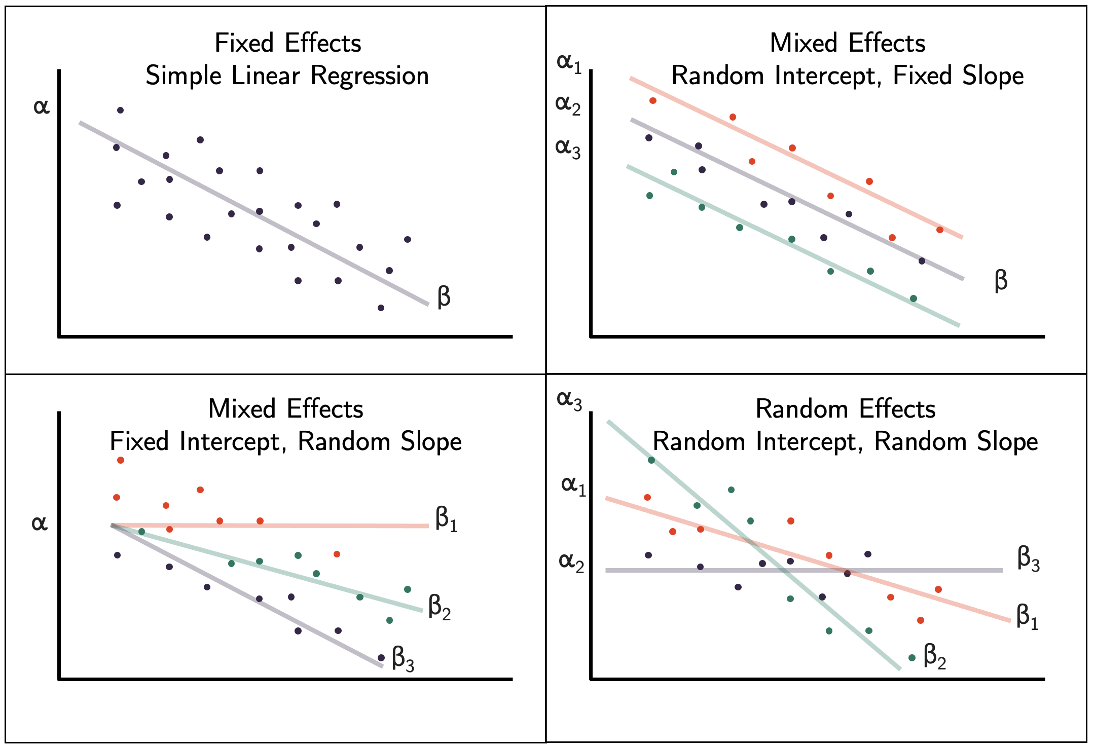
Source: https://bookdown.org/steve_midway/DAR/random-effects.html
3.3 Fixed effect regression approach
One might account for the nested structured of the data by including a “grouping variable” for individuals (e.g. dummy for each country) or inclusion of contextual explanatory variables (e.g. gender equality index per country).
\[y_{ij}=\beta_0 + \beta_1*X_{ij} + \sum^{}_{C-1}(\beta_C*CD_j + \epsilon_{ij})\]
- \(\beta_0\) is the overall intercept (e.g. reference country)
- \(\beta_C\) is the intercept for one country
Problem: grouping parameters are treated as fixed effects ignoring random variability associated with macro-level characteristics. This “dummy variable approach” thus suggests that group differences are fixed effects.
3.4 Random intercept model (with fixed slope)
In its simplest form, a MLM is in the form of a “null model” which contains no explanatory variables.
It thus includes one regression constant (intercept) and assumes that this varies across contexts.
So far, we are able to answer questions like:
- Are there countries differences with respect to happiness?
- How much of this variation is due to these country differences?
4 Interclass Correlation Coefficient (ICC)
4.1 Definition and recommendation
A MLM with a random intercept is a point where we can pause and run a diagnostic called the Interclass Correlation Coefficient (ICC):
\[ICC = \frac{\sigma^2_\alpha}{\sigma^2+\sigma^2_\alpha}\]
where \(\sigma^2_\alpha\) is the variance due to groups.
The ICC tells us how much similarity is within contexts (i.e. countries). Basically, it accounts for the closeness of observations in same context relative to closeness of observations in different contexts.
Practical recommendation:
The ICC ranges from 0 (no clustering/single level data structure) and 1 (maximum clustering). In practice, 0 or 1 rarely occur. A general recommendation is that if the ICC is small, then use of a single level model.
5 Models in details
5.1 Random intercept model (with fixed slope) including one predictor
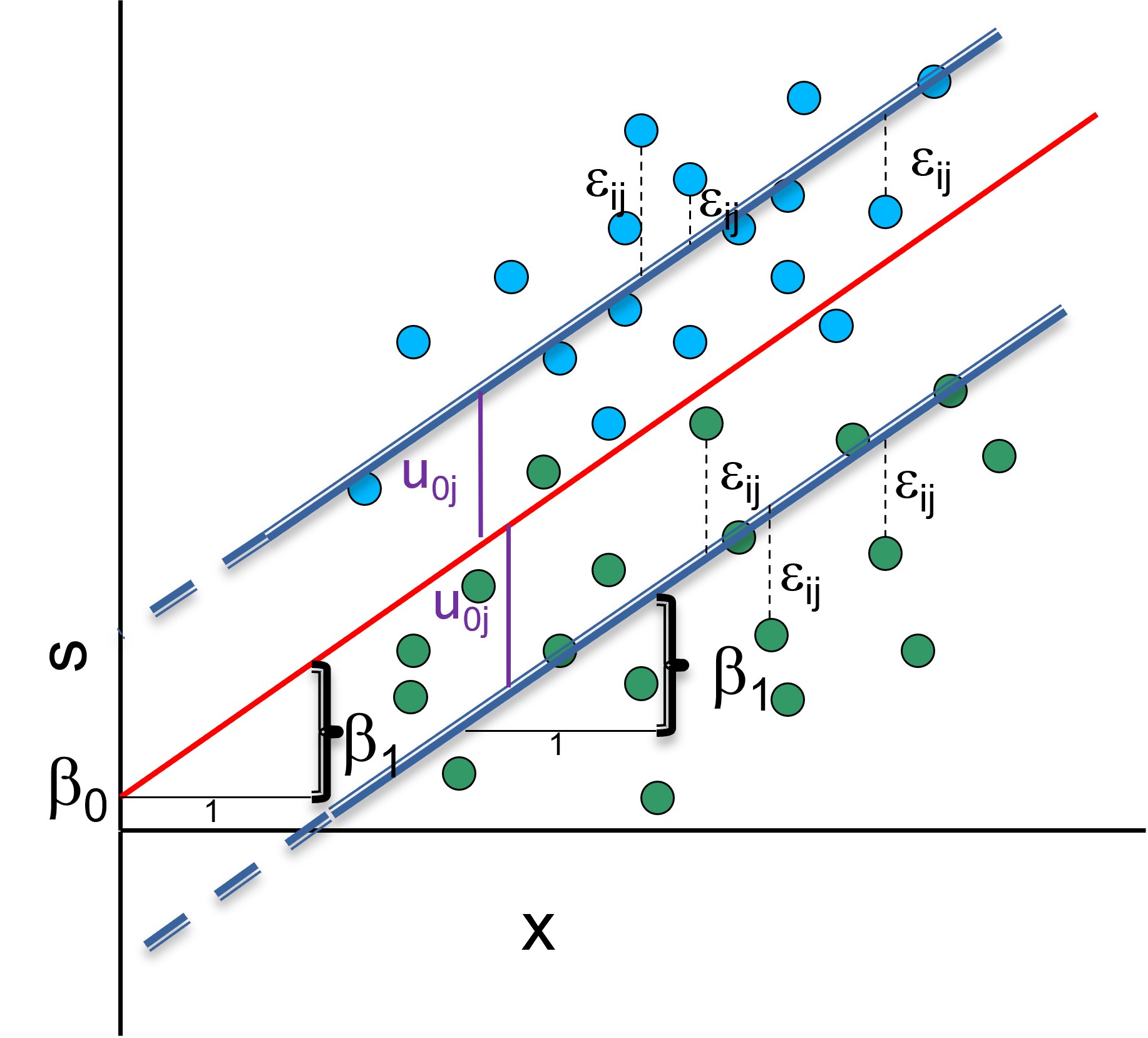
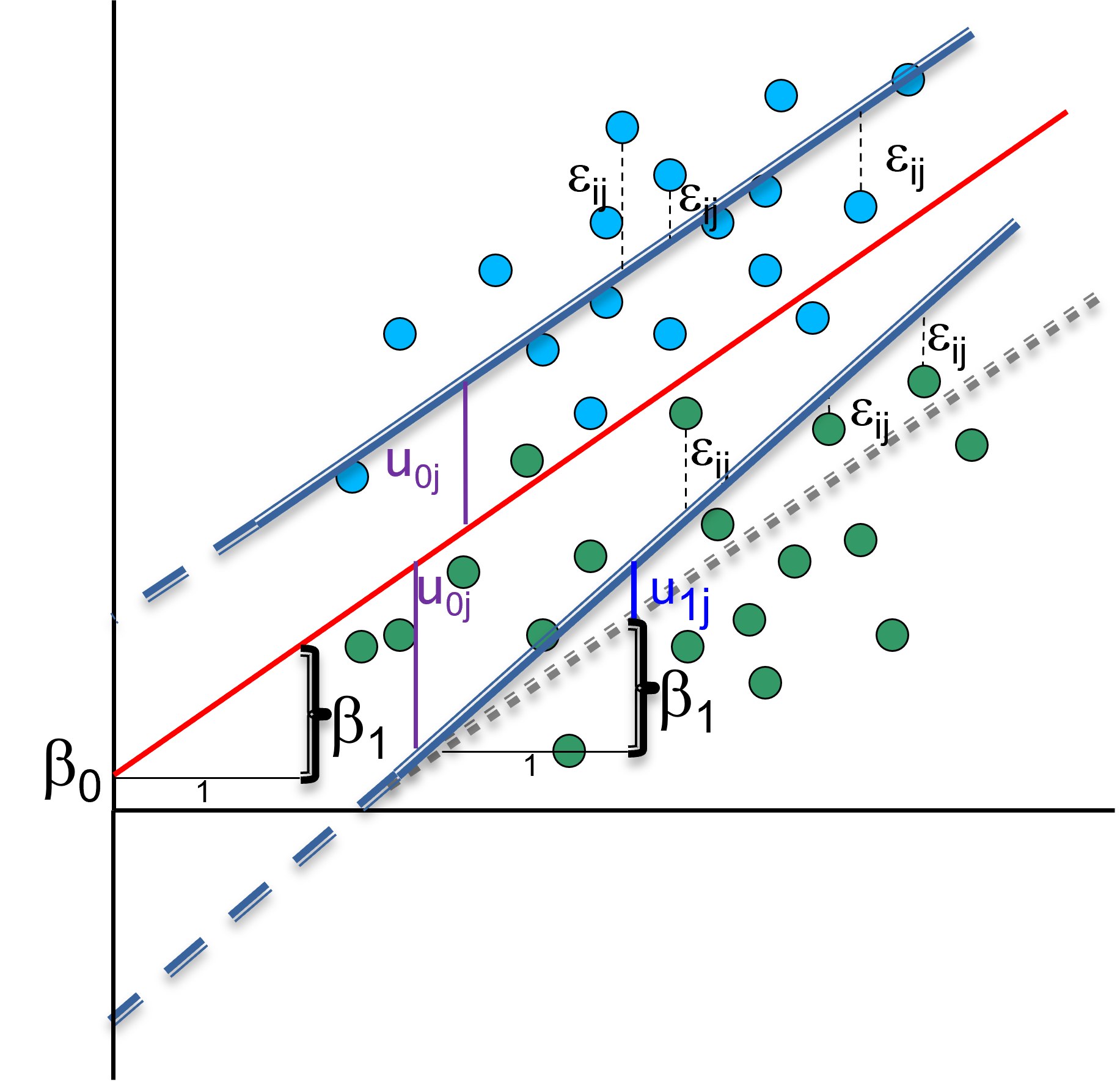
Random intercept model is a combination of variance component and a linear model (for a person \(i\) in country \(j\)): \(y_{ij}=\beta_0 + \beta_x*X_{ij} + u_{0j} + \epsilon_{ij}\).
- \(\beta_0 + \beta_x*X_{ij}\) is the fixed part
- \(u_{0j} + \epsilon_{ij}\) the random part
There are two random terms and therefore two types of residuals: \(u_j\) a the level-2 and \(e_{ij}\) at the level-1. There are also an overall (average) line \(β_0\) and group (average) lines \(β_0+u_j\).
5.2 What we can answer so far
So far, we are able to answer questions as:
- Do country differences in happiness remain after controlling for gender?
- How much of variation in happiness is due to country differences after controlling for gender?
Limitations:
The assumption of random intercept model suggests that group lines have all same slope as overall regression line in every group (effect of X on Y is the same for every country).
Is this always valid?
It can be argued that X is not a fixed but a random effect and that its slope can vary across groups.
5.3 Random slope model (with random intercept)
We can account for the random slope by adding random term to coefficient of \(x_{1ij}\) (e.g. working hours), so it can be different for each group (e.g. country): \(y_{ij} = \beta_0 + (\beta_1 + u_{1j})*x_{1ij} + u_{0j} + \epsilon_{0ij}\)
If you have no reasons to expect the effect of your level-1 predictor to vary between clusters, the random intercept model is more appropriate than a random slope model. You can also formally test which of the model is better.
With a random slope model, we could now answer questions as: Does the effect of being employed has the same impact on happiness across countries?
5.4 Note: fixed intercept with random slope
It might be the case that a model requires a fixed intercept but a random slope specification.
This could be the case when we hypothesize that the effect of our predictor differs among groups, but when we want to fix the intercept because we know that all groups start in a similar place.
6 Cross-level interactions
6.1 Link between individual and contextual factors
Adding cross-level interactions allows us to assess whether contextual factors (Z) influence the effect of level-1 X variables.
For instance, we can answer questions such as:
- Is the effect of gender on happiness stronger/weaker in countries with a high gender equality index?
The cross-level interaction should be included in the fixed part of model:
\[ y_{ij} = \beta_0 + \beta_1*x_{ij} + \beta_2*Z_j + \beta_3*x_{ij}Z_j + u_{0j} + u_{1j}x_{ij} + \epsilon_{ij} \]
Therefore, the direct main and interaction effects have to be interpreted together (similar to OLS).
7 Variance decomposition approach
7.1 Hox’s approach
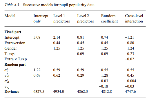
Hox (2010, pp.70) proposes to examine residual error variance in a sequence of models:
Interpretation and calculation:
- \(\sigma_{e}^2\): variance of the pupil-level residual errors
- \(\sigma_{u0}^2\): variance of the class-level residual errors
- \(\sigma_{u2}^2\): variance of the residual errors \(u_{2j}\)
- ICC = \(\frac{\sigma_{u0}^2}{(\sigma_{u0}^2 + \sigma_{e}^2)}=\frac{0.69}{(0.69+1.22)} = 0.36\). Thus, 36% of the variance of the popularity scores is at the group level, which is very high.
8 Centering and standardizing
8.1 Group and grand mean centering
The regression intercept equals the expected value of Y if all X are 0.
What if 0 has no useful meaning or is not possible (e.g. age of 0)? In this case, it is useful to transform the X variables, for instance by centering them.
There are two options:
- Grand mean centering: computing variables as deviations from the overall mean (the constant in model reflects the mean of all cases)
- Group mean centering: computing variables as deviation from the group mean (decomposes within vs. between effects)
8.2 Interpretation
Imagine you have the following two-level null model specified for a dependent variable \(Y_{ij}\) (where \(i\) represent students and \(j\) schools):
- Level 1 (students): \(Y_{ij} = b_{0j} + r_{ij}\)
- Level 2 (schools): \(b_{0j} = g_{00} + u_{0j}\)
In these equations:
- \(b_{0j}\) represents the group-mean of Y
- \(r_{ij}\) represents level-1 residuals
- \(g_{00}\) represents the grand mean of the variable Y
- \(u_{0j}\) represents the group-specific deviation from the grand mean of Y
9 Empirical example in R
9.1 Example
Let’s prepare survey data to analyse citizens’ happiness using the round 10 of the European Social Survey.
library(foreign)
db <- read.spss(file=paste0(getwd(),"/data/ESS10.sav"),
                use.value.labels = T,
                to.data.frame = T)
sel <- db |>
  dplyr::select(cntry,happy,pdwrk,wkhtot,gndr,agea,eduyrs) |>
  stats::na.omit()
# recodings
sel$happy <- as.numeric(sel$happy)
sel$wkhtot <- as.numeric(sel$wkhtot)
sel$work <- ifelse(sel$pdwrk=="Marked","1","0")
sel$gndr <- as.factor(sel$gndr)
sel$eduyrs <- as.numeric(sel$eduyrs)
sel$agea <- as.numeric(sel$agea)
sel$cntry <- droplevels(sel$cntry)
9.2 Country dummies model
Let’s make a model to predict the difference in happiness explained by gender and including country dummies:
 [1] "================================================"
 [2] "                         Dependent variable:    "
 [3] "                     ---------------------------"
 [4] "                                happy           "
 [5] "------------------------------------------------"
 [6] "gndrFemale                0.060*** (0.023)      "
 [7] "cntrySwitzerland          1.862*** (0.062)      "
 [8] "------------------------------------------------"
 [9] "Observations                   26,404           "
[10] "R2                              0.092           "
[11] "Adjusted R2                     0.091           "
[12] "Residual Std. Error      1.824 (df = 26384)     "
[13] "F Statistic          140.294*** (df = 19; 26384)"
[14] "================================================"
[15] "Note:                *p<0.1; **p<0.05; ***p<0.01"
9.3 Null model and ICC
mixed <- lme4::lmer(happy ~ 1 + (1 | cntry),
                    data=sel)
stargazer::stargazer(mixed,
                     type="text",
                     single.row = T)
===============================================
                        Dependent variable:
                    ---------------------------
                               happy
-----------------------------------------------
Constant                 8.348*** (0.133)
-----------------------------------------------
Observations                  26,404
Log Likelihood              -53,390.860
Akaike Inf. Crit.           106,787.700
Bayesian Inf. Crit.         106,812.300
===============================================
Note:               *p<0.1; **p<0.05; ***p<0.01
The intercept of 8.34 in this model is simply the average happiness across all individuals and countries.
ICC = 0.33/(3.32+0.33)=0.09, thus 9% of variance in happiness is it due to belonging to a different country and 91% due to individual characteristics.
9.4 Random intercept model
The effect of gender on happiness can be included in the regression model with the countries as random intercepts:
random <- lme4::lmer(happy ~ 1 + gndr +
                       (1 | cntry),
                     data=sel)
stargazer::stargazer(random,
                     type="text",
                     single.row = T)
===============================================
                        Dependent variable:
                    ---------------------------
                               happy
-----------------------------------------------
gndrFemale               0.059*** (0.023)
Constant                 8.316*** (0.134)
-----------------------------------------------
Observations                  26,404
Log Likelihood              -53,390.270
Akaike Inf. Crit.           106,788.500
Bayesian Inf. Crit.         106,821.300
===============================================
Note:               *p<0.1; **p<0.05; ***p<0.01
Interpretation:
- average expected happiness score for a person is 8.3 across all countries
- women are on average more happy (0.06)
library(magrittr)
library(tibble)
model_coefs <- coef(random)$cntry
colnames(model_coefs) = c("Intercept","Slope")
print(head(model_coefs))
Intercept Slope
Bulgaria 7.211262 0.0594652
Switzerland 9.063355 0.0594652
Czechia 7.937866 0.0594652
Estonia 8.485431 0.0594652
Finland 9.136284 0.0594652
France 8.426651 0.05946529.5 Multiple explanatory variables
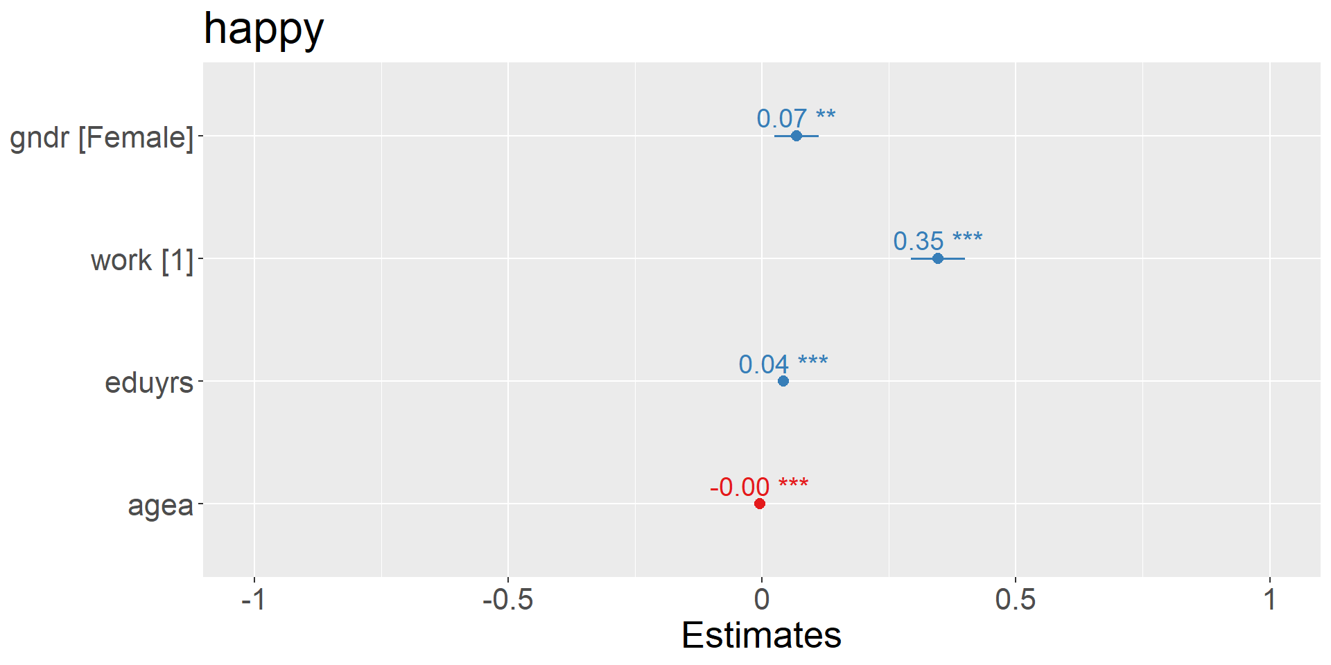
We can more explanatory variables in the regression model:
random2 <- lme4::lmer(happy ~ 1 + gndr +
                        work + eduyrs + agea +
                        (1 | cntry),
                      data=sel)
stargazer::stargazer(random2,
                     type="text",
                     single.row = T)
===============================================
                        Dependent variable:
                    ---------------------------
                               happy
-----------------------------------------------
gndrFemale               0.068*** (0.022)
work1                    0.347*** (0.027)
eduyrs                   0.043*** (0.003)
agea                     -0.004*** (0.001)
Constant                 7.624*** (0.140)
-----------------------------------------------
Observations                  26,404
Log Likelihood              -53,052.490
Akaike Inf. Crit.           106,119.000
Bayesian Inf. Crit.         106,176.200
===============================================
Note:               *p<0.1; **p<0.05; ***p<0.01
The average expected happiness for a person is 7.6 across all countries.
It varies by a score of 0.30 between countries and by a score of 3.24 within countries.
       grp        var1 var2      vcov     sdcor
1    cntry (Intercept) <NA> 0.3010224 0.5486551
2 Residual        <NA> <NA> 3.2413796 1.8003832
Further interpretation:
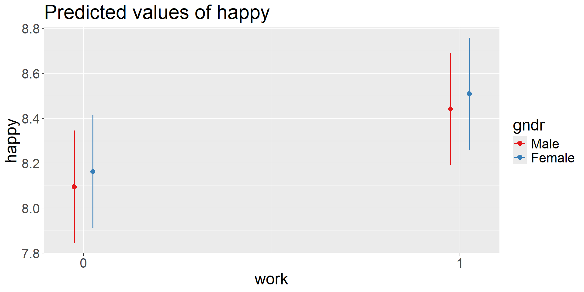
- working increases the happiness on average by 0.34 points
- 1 year more of education increase happiness by 0.04 points
9.6 Random slope model
randomslope <- lme4::lmer(happy ~ 1 + gndr +
                            work + eduyrs + agea +
                            (1 + work| cntry),
                          data=sel)
stargazer::stargazer(randomslope,
                     type="text",
                     single.row = T)
===============================================
                        Dependent variable:
                    ---------------------------
                               happy
-----------------------------------------------
gndrFemale               0.074*** (0.022)
work1                    0.318*** (0.066)
eduyrs                   0.043*** (0.003)
agea                     -0.003*** (0.001)
Constant                 7.630*** (0.167)
-----------------------------------------------
Observations                  26,404
Log Likelihood              -52,992.340
Akaike Inf. Crit.           106,002.700
Bayesian Inf. Crit.         106,076.300
===============================================
Note: *p<0.1; **p<0.05; ***p<0.01 grp var1 var2 vcov sdcor
1 cntry (Intercept) <NA> 0.45567493 0.6750370
2 cntry work1 <NA> 0.06807283 0.2609077
3 cntry (Intercept) work1 -0.14743662 -0.8371261
4 Residual <NA> <NA> 3.22358950 1.7954357- the average happiness for a person is 7.6 across all countries (varies by a score of 0.45 between countries)
- being employed increase the happiness on average by 0.32 (varies by a score of 0.06 between countries)
- the correlation between the intercept and slope is negative (-0.14) thus suggesting that in “happy” countries the average effect of work on happiness is lower.
9.7 Visualizations: coefficients & marginal effects

Multivariate statistics
