library(foreign)
db <- read.spss(file=paste0(getwd(),
                "/data/1184_Selects2019_Panel_Data_v4.0.sav"),
                use.value.labels = T,
                to.data.frame = T)
sel <- db |>
  dplyr::select(W3_f11100,W3_f12800c,
                W2_f13400a,W2_f13400b,W2_f13400c,W2_f13400d,
                W2_f13400e,W2_f13400f) |>
  stats::na.omit() |>
  dplyr::rename("particip"="W3_f11100",
                "party_trust"="W3_f12800c",
                "tv"="W2_f13400a",
                "newsp"="W2_f13400b",
                "freen"="W2_f13400c",
                "socmed"="W2_f13400d",
                "online"="W2_f13400e",
"radio"="W2_f13400f") Moderation analysis presentation
Learn what moderation analysis is and how to run the analysis in R
1 Moderation analsyis
1.1 Definition
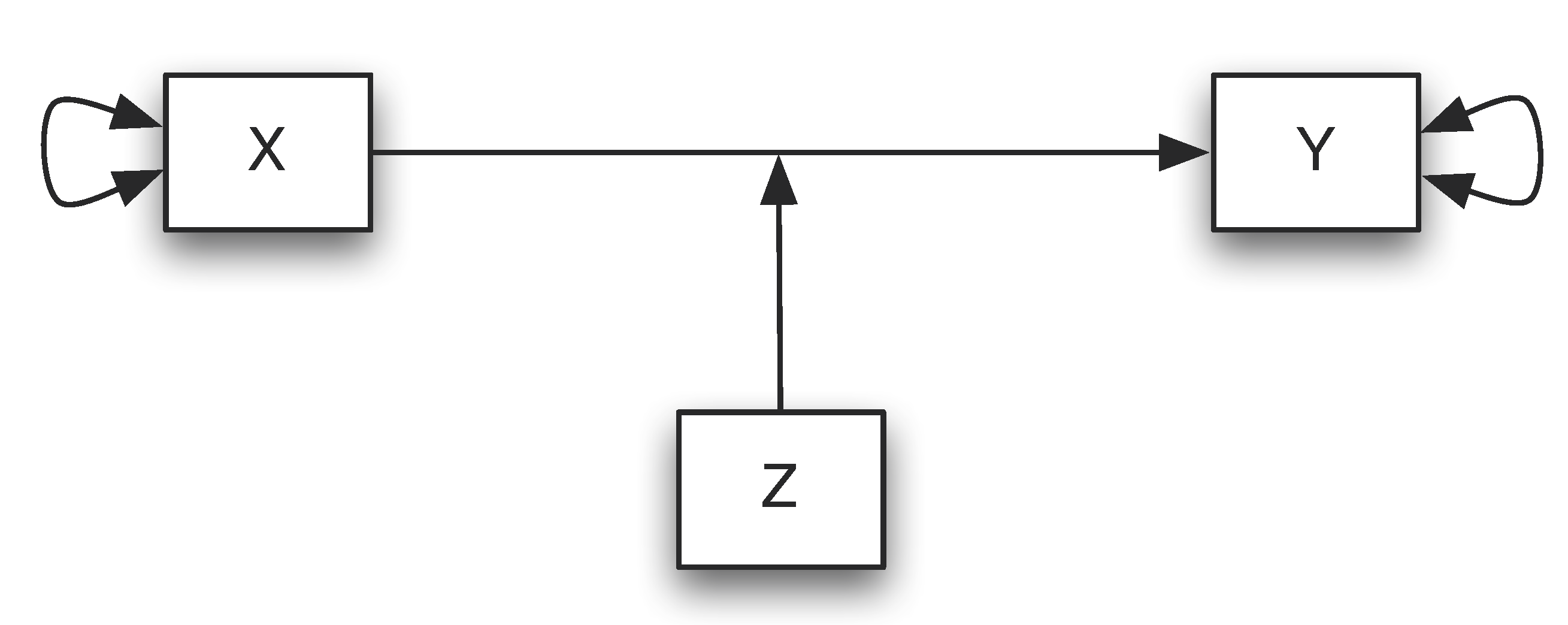
Moderation analysis allows us to test for the influence of a third variable, Z, on the relationship between variables X and Y. Rather than testing a causal link between these other variables, moderation tests for when or under what conditions an effect occurs.

1.2 Interaction
Moderators can strengthen, weaken, or reverse the nature of a relationship. Moderation can be tested by looking for significant interactions between the moderating variable (Z) and the independent variable (X).
Nota bene: Moderators (when) are conceptually different from mediators (how/why) but some variables may be a moderator or a mediator depending on your question.
1.3 Similarity with ANOVA
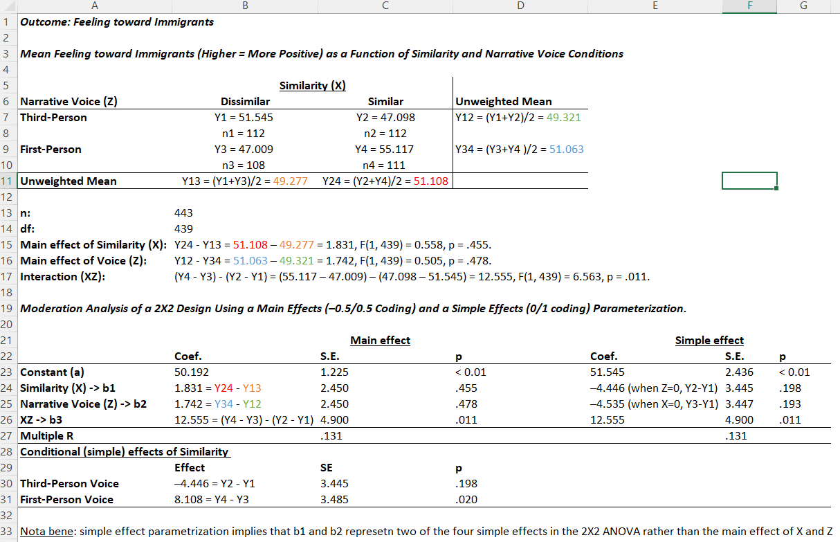
The moderation is an interaction and therefore comparable to the interaction in ANOVA. If X and moderator are dichotomous, the moderation corresponds to a 2x2 ANOVA.
However, a moderator moderates the causal relationship from X to Y. The scale level can be dichotomous, categorical or metric. Furthermore, a moderator must be causally independent of X.
1.4 Illustration
See Igartua and Hayes (2021) for a complete discussion.
1.5 How-To
Technically, moderations (interactions) are linked multiplicatively in the regression analysis: A x B.
Statistically, the moderator and X must always be considered “in isolation” (not just as moderation or interaction).
Moderation analysis can be conducted by adding one (or multiple) interaction terms in a regression analysis. For example, if Z is a moderator for the relation between X and Y, we can fit a regression model:
\[ Y = \beta_{0} + \beta_{1}*X + \beta_{2}*Z + \beta_{3}*XZ + \epsilon \]
\[ Y = \beta_{0} + \beta_{2}*Z + (\beta_{1} + \beta_{3}*Z)*X + \epsilon \]
Thus, if \(\beta_{3}\) is not equal to 0, the relationship between X and Y depends on the value of Z, which indicates a moderation effect.
1.6 Binary moderator
\[ Y = \beta_{0} + \beta_{2}*Z + (\beta_{1} + \beta_{3}*Z)*X \]
If Z is a dichotomous/binary variable (e.g. gender) the above equation can be written as:
\[ \beta_{0} + \beta_{1}*X + \epsilon \] for male (Z=0)
\[ \beta_{0} + \beta_{2} + (\beta_{1} + \beta_{3})*X + \epsilon \] for female (Z=1)
2 Interpretation and centering
2.1 Interpretation
If X and/or moderator become significant, main effects are present. If the moderation term becomes significant, there is a moderation effect. The (possibly significant) influences of X and the moderator are then so-called “conditional” effects.
The value 0 usually has no meaningful meaning (e.g. in rating scales 1 to 5 there is no zero at all). Therefore, it is a good practice to centering means subtracting the overall mean from each value.
2.2 Effect of centering on the interpretation
The change in meaning must be taken into account in the interpretation:
- influence of the predictor on Y with an average expression of the moderator
- influence of the moderator on Y with an average expression of the predictor
2.3 Variable’s effect as a function of a moderator
Let’s assume that X and Z are either dichotomous or continuous and the outcome variable Y is a continuous dimension suitable for analysis with linear regression, we have the following equations:
\[ \hat{Y} = a + b_1*X + b_2*Z + b_3*XZ = a + (b_1+b_3*Z)*X + b_2*Z\]
In this representation, the weight for X is not a single number but, rather, a function of Z: \(b_1+b_3*Z\).
The output is sometimes called the simple slope of X or the conditional effect of X.
The coefficients \(b_1\) and \(b_2\) may or may not have a substantive interpretation, depending on how X and Z are coded or, in the case of dichotomous X and Z, what two numbers are used to represent the groups in the data.
2.4 Correct interpretations
- \(b_1\) is the conditional effect of X on Y when Z = 0.
- \(b_1\) is the estimated difference in Y between two cases in the data that differ by one unit in X but have a value of 0 for Z.
- \(b_2\) is the conditional effect of Z on Y when X = 0.
- When X = 0, the conditional effect of Z reduces to \(b_2\).
- When Z = 0, X’s effect equals \(b_1\); when Z = 1, X’s effect equals \(b_1+b_3\); when Z = 2, X’s effect is \(b_1+2b_3\), and so forth.
2.5 Multicollinearity
The moderation term is formed with moderator and X. However, the moderator and X are also contained individually in the regression equation. This often leads to multicollinearity (i.e. low tolerances or high VIF values).
If moderator and X are centered, the symptoms of multicollinearity are superficially defused. However, the multicollinearity itself remains.
Multicollinearity means that predictors are (too strongly) related to each other. Since the moderation term also consists of A (or B), it can easily correlate with A (or B).
3 Visualization of the moderation effect
3.1 Simple slopes
When the moderation effect becomes significant, it needs to be “illustrated” in order to make it interpretable. To do so, we can rely on simple slope analysis: comparison of the regression lines for low, medium and high levels of the moderator.
Typically, we use the mean value of the moderator, as well as the values + and - 1 SD are used, but theoretically any values can be considered.

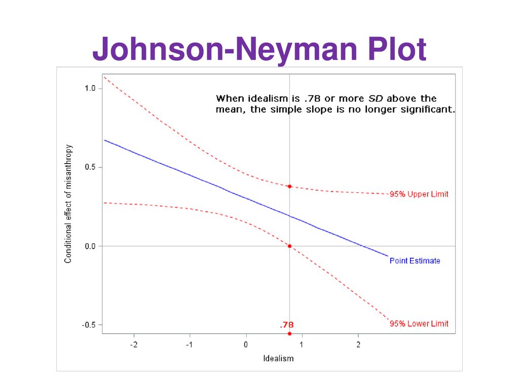
3.2 Significance range: Johnson & Neyman
This method suggests to conduct comparison of the regression equation for many characteristics of the moderator to identify areas of significance.
It is more useful than simple slopes for metric moderators, since illustrations result in less loss of information in the moderator’s levels. The effect (b) of the X on Y is now illustrated in the diagram as a function of the moderator (not to be confused with a regression line!), as well as the confidence interval for this effect:

4 Steps in the analysis
4.1 Five main steps
A moderation analysis typically consists of the following steps:
- compute the interaction term X*Z
- fit a multiple regression model with X, Z, and XZ as predictors
- test whether the regression coefficient for XZ is significant or not
- interpret the moderation effect
- display the moderation effect graphically.
5 Example in R
5.1 Example: news attention as moderator
For example, trust in politicians (e.g., trust in national parties) could moderate the effect of citizens’ media diet (e.g., attention to political news) on political participation in election.
We will be using the Selects Swiss Panel Election Study 2019 and the following variables:
- participation (in W3): W3_f11100
- trust in politicians (in W3, assumed similar in W2): W3_f12800c
- media diet (in W2): W2_f13400a-f
5.2 Prepare the data
Let’s load the data and select the relevant variables:
5.3 Recoding and creation of media score
# recode participation
sel$particip <- ifelse(sel$particip=="Voted",1,0)
sel$particip <- as.factor(sel$particip)
# trust as numeric
sel$party_trust <- as.character(sel$party_trust)
sel$party_trust[sel$party_trust=="Full trust"] <- "10"
sel$party_trust[sel$party_trust=="No trust"] <- "0"
sel$party_trust <- as.numeric(sel$party_trust)
# trust as binary
sel$party_trust_b <- ifelse(sel$party_trust>=6, "yes","no")
# reverse scale for media attention and build score
sel$tv <- (as.numeric(sel$tv)-4)*(-1)
sel$newsp <- (as.numeric(sel$newsp)-4)*(-1)
sel$freen <- (as.numeric(sel$freen)-4)*(-1)
sel$socmed <- (as.numeric(sel$socmed)-4)*(-1)
sel$online <- (as.numeric(sel$online)-4)*(-1)
sel$radio <- (as.numeric(sel$radio)-4)*(-1)
sel$medatt <- (sel$tv+sel$newsp+sel$freen+sel$socmed+sel$online+sel$radio)/6
5.4 Variable centering
When Z and X are numeric, it is important to mean center both your moderator and your independent variable to reduce multicolinearity and to make interpretation easier. Centering can be done using the scale() function, which subtracts the mean of a variable from each value in that variable.
5.5 Moderation model
We can compute moderation analysis directly with the glm() function but we can also rely on the PROCESS macro developed by Hayes. You can download PROCESS for R here.
mod1 <- glm(particip ~
              party_trust + medatt +
              party_trust*medatt,
            data=sel,
            family = "binomial")
stargazer::stargazer(mod1, type="text", single.row = T)
==============================================
                       Dependent variable:
                   ---------------------------
                            particip
----------------------------------------------
party_trust             0.095*** (0.022)
medatt                  0.895*** (0.084)
party_trust:medatt       -0.071* (0.041)
Constant                1.450*** (0.042)
----------------------------------------------
Observations                  3,940
Log Likelihood             -1,902.390
Akaike Inf. Crit.           3,812.780
==============================================
Note: *p<0.1; **p<0.05; ***p<0.015.6 PROCESS output
********************* PROCESS for R Version 4.3.1 *********************

           Written by Andrew F. Hayes, Ph.D.  www.afhayes.com
   Documentation available in Hayes (2022). www.guilford.com/p/hayes3

***********************************************************************

PROCESS is now ready for use.
Copyright 2020-2023 by Andrew F. Hayes ALL RIGHTS RESERVED
Workshop schedule at http://haskayne.ucalgary.ca/CCRAM
********************* PROCESS for R Version 4.3.1 *********************

           Written by Andrew F. Hayes, Ph.D.  www.afhayes.com
   Documentation available in Hayes (2022). www.guilford.com/p/hayes3

***********************************************************************

Model : 1
    Y : particip
    X : medatt
    W : party_trust

Sample size: 3940


***********************************************************************
Outcome Variable: particip

Coding of binary Y for logistic regression analysis:
   particip  Analysis
     0.0000    0.0000
     1.0000    1.0000

Model Summary:
       -2LL   ModelLL        df         p  McFadden  CoxSnell  Nagelkrk
  3804.7804  163.2159    3.0000    0.0000    0.0411    0.0406    0.0639

Model:
                coeff        se         Z         p      LLCI      ULCI
constant       1.4497    0.0422   34.3543    0.0000    1.3670    1.5324
medatt         0.8947    0.0838   10.6791    0.0000    0.7305    1.0589
party_trust    0.0951    0.0219    4.3329    0.0000    0.0521    0.1381
Int_1         -0.0713    0.0411   -1.7357    0.0826   -0.1517    0.0092

These results are expressed in a log-odds metric.

Product terms key:
Int_1  :  medatt  x  party_trust

Likelihood ratio test of highest order
unconditional interaction(s):
       Chi-sq        df         p
X*W    3.0448    1.0000    0.0810
----------
Focal predictor: medatt (X)
      Moderator: party_trust (W)

Conditional effects of the focal predictor at values of the moderator(s):
  party_trust    effect        se         Z         p      LLCI      ULCI
      -1.6830    1.0146    0.1050    9.6611    0.0000    0.8087    1.2204
       0.3170    0.8721    0.0856   10.1847    0.0000    0.7042    1.0399
       2.3170    0.7296    0.1308    5.5762    0.0000    0.4731    0.9860

******************** ANALYSIS NOTES AND ERRORS ************************

Level of confidence for all confidence intervals in output: 95

W values in conditional tables are the 16th, 50th, and 84th percentiles.
5.7 Visualizations
The plot_model() function will automatically plot the simple slopes (1 SD above and 1 SD below the mean) of the moderating effect:
5.8 Moderator as categorical variable
We use a dichotomous moderator and check whether we obtain similar results:
===================================================
                            Dependent variable:
                        ---------------------------
                                 particip
---------------------------------------------------
party_trust_byes             0.364*** (0.084)
medatt                       1.048*** (0.119)
party_trust_byes:medatt       -0.287* (0.167)
Constant                     1.247*** (0.061)
---------------------------------------------------
Observations                       3,940
Log Likelihood                  -1,904.162
Akaike Inf. Crit.                3,816.324
===================================================
Note:                   *p<0.1; **p<0.05; ***p<0.01

Multivariate statistics


