EFA and CFA

Recap session

1 EFA versus CFA

1.1 Main differences between both approaches

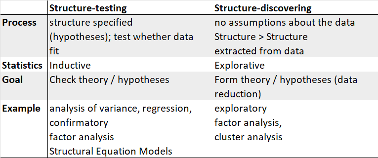
In EFA, all measured variables are related to every latent variable. It is used to reduce data to a smaller set of summary variables and to explore the underlying theoretical structure of the phenomena. Therefore, it requires interpretation.

In CFA, researchers can specify the number of factors required in the data and which measured variable is related to which latent variable. It asks how well a proposed model fits a given data. It does not give a definitive answer, but compares models (and data).

1.2 Prerequisites and guidelines

Main prerequisites:

• Condition: There are several interval-scaled characteristics (items).
• Rule of thumb: At least 50 people and 3x more people as variables (ideally: 5x more people as variables!).

Guidelines:

• Factor analysis does not play well with missing data: it is better to remove cases that have missing data.
• Factor analysis is designed for continuous data (although it is possible to include categorical data with other methods).

2 Factors and representation

2.1 Why use dimensionality reduction?

Dimensionality reduction transforms a data set from a high-dimensional space into a low-dimensional space.

It is useful when there are too many variables to achieve a good understanding (or visualization) of the data.

Another issue is multicollinearity: predictors may be measuring the same latent effect(s), and thus such predictors will be highly correlated.

• Factor/dimension: latent dimension responsible for the manifestation of a directly measured variable

• Indicator/item: a directly measured variable that, together with other variables, makes up a factor/dimension

2.2 Fundamental theorem

In EFA, each item cannot be fully explained by a linear combination of the factors:

\[Z_{ij} = f_{i1}a_{1j} + f_{i2}a_{2j} + ... + f_{ip}a_{pj} + e_j\] e.g. prejudice = some items + residuals

The variance can be partitioned into common and unique variance:

• Common variance: amount of variance that is shared among a set of items (communality).
• Unique variance: any portion of variance that is not common.
  • Specific variance: variance that is specific to a particular item
  • Error variance: comes from errors of measurement

2.3 Important concepts

• Factor loading: correlation coefficient between the item and the factor (angle between the factor and a given item)
• Squared factor loading: percent of variance in a given item explained by the factor
• Factor eigenvalue: proportion of the variance of all directly measured items that is explained by a factor
  
• Item communality: proportion of the variance of an item that is explained by all factors

Original output from Hidayat et al. (2018).

3 EFA procedure

3.1 Step 1) and procedures in EFA

Step 1) suitability of the data:

• Aim: only relevant items should be included in the factor analysis.
• Tools:
  • Have a look at the correlation matrix.
  • Use the Bartlett’s test of Sphericity:
    • H0: The variables are uncorrelated in the population
    • H1: The variables are correlated in the population
  • Kaiser-Meyer-Olkin criterion (KMO)
    • test to what extent the variance of one variable is explained by the other variables (values from .8 desirable)

psych::cortest.bartlett(data)
psych::KMO(data)

3.2 Step 2) and procedures in EFA

Step 2) choice of the number of factors:

• Aim: extract the most relevant number of factors given the items
• Tools:
  • Kaiser criterion: identifies the number of factors that explains more variance than any of the original variables (eigenvalue of 1 onwards: “how much variance each factor accounts for in your data”)
  • Scree plot: eigenvalues are plotted in the graphic and the factors that lie above a “threshold” are extracted
  • Content plausibility or a priori criterion

# eigenvalue method (Kaiser's rule)
ev <- eigen(cor(sel)) 
print(ev$values)
# scree plot method
psych::scree(sel, pc=FALSE) 

3.3 Step 3) and procedures in EFA

Step 3) choice of the type of rotation:

• Aim: obtaining a simple structure to relieve the factor interpretation.
• Types of rotations:
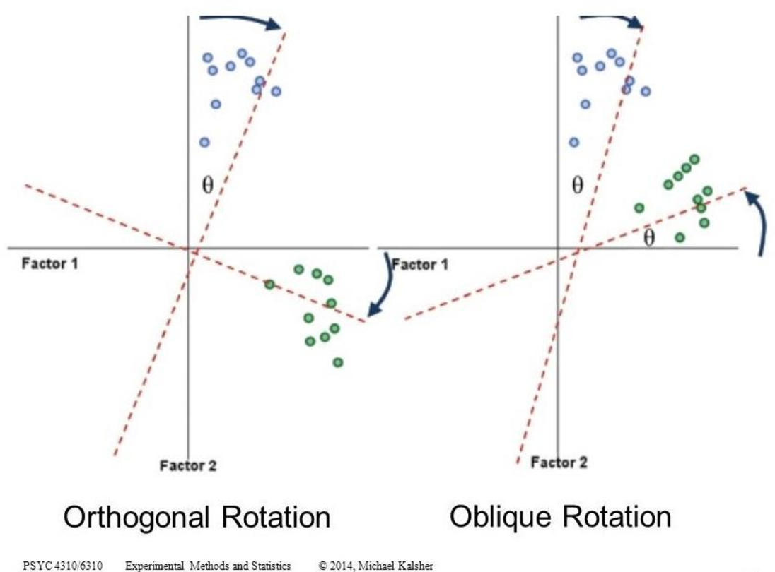
  • Orthogonal (Right Angle): the factor are uncorrelated
  • Oblique: the factor are correlated

What is the difference?

Solution

In an oblique rotation factors are correlated. We account for the angle of axis rotation and for the angle of correlation.

fit_oblique <- psych::fa(data, 
                         nfactors=4, 
                         rotate="oblimin")
fit_orthogonal <- psych::fa(data, 
                            nfactors=4, 
                            rotate="varimax")

3.4 Step 4) and procedures in EFA

Step 4) evaluation of the results and possibly repeat 2) & 3):

• Aim: interpret the factors.
• Process:
  • loadings from .5 are usually interpreted
  • ideally, variables load exactly high on one factor and low on another
  • variables with higher loadings should be given more consideration in naming the factors
  • negative charge must be taken into account in the interpretation of the factors
  • also consider the total variance explained by the factors and the respective contribution of each factor

summary(fit)
print(fit$loadings, digits=2, cutoff=0.3, sort=TRUE)

3.5 Interpretation: loadings > 1

Factor loadings can be greater than 1. Especially with highly correlated factors.

“This misunderstanding probably stems from classical exploratory factor analysis where factor loadings are correlations if a correlation matrix is analyzed and the factors are standardized and uncorrelated (orthogonal). However, if the factors are correlated (oblique), the factor loadings are regression coefficients and not correlations and as such they can be larger than one in magnitude.” (Jöreskog, 1999)

3.6 Step 5) and procedures in EFA

Step 5) interpret and write-up results:

• Process:
  • display the results (visualization)
  • name the factors and assess there theoretical relevance
  • assess the coherence of the factors (internal validity) using Cronbach’s alpha (varies between 0 and 1: ideally alpha>0.70).

# visualization
loads <- fit2$loadings
psych::fa.diagram(loads)
# coherence of the factors (internal validity)
# check.keys=T allows to reverse negative loadings
alpha_f1 = psych::alpha(f1, check.keys=T) 
print(alpha_f1$total)

3.7 EFA example: Schulz et al. (2018)

• Factor loading: correlation coefficient between the item and the factor (angle between the factor and a given item)
• Item communality (\(h^2\): proportion of the variance of an item that is explained by all factors

4 CFA procedure

4.1 Purpose of CFA

CFA is a model-data fit test based on multivariate regression. Outputs are coefficients of paths and fit indices.

Items that should theoretically load on a factor should correlate empirically (if not, they are probably not determined by the same factor). The model-theoretical covariance matrix as defined by the measurement model should faithfully reproduce the empirical covariance matrix.

Problem: question of whether a system of equations can be solved mathematically, which means that the model parameters (free parameters) must be estimated from the empirical variances and covariances of the manifest variables.

Logic: factor loadings, error terms, factor variance, and, if applicable, permitted correlations between factors must be calculable/representable with the help of empirical parameters.

Model identification: if all parameters are to be estimated in the model, then the model is identified. If not, the model is not solvable (“too many unknowns”) and it is unidentified.

4.2 Model identification and structure

The model identification is about determining the degrees of freedom of the model.

To do so, we need to understand the different types of parameters:

• Fixed parameters: are assigned a specific constant value a priori.
• Constrained parameters: are estimated in the model, but have values corresponding exactly to the value of one or more other parameters.
• Free parameters: are considered unknown and should be estimated from the empirical data.

Identifying the model structure is conducted in two “tasks”:

• every factor should be given a metric to be identified (see marker method versus variance standardization method)
• checking whether there is enough information to estimate the model

4.3 Degree of freedom

If n manifest items are collected within the framework of a project, then the empirical variances and covariances of these variables can be calculated:

\[ p = \frac{n(n+1)}{2} \]

p corresponds to the number of non-redundant values in the variance-covariance matrix (available “information” for calculating all free parameters of our model).

The degree of freedom of the model (\(df_M\)) is expressed as the difference between the available empirical information (p) and the number of parameters to be estimated (q):

\[ df_M = p - q \]

4.4 Under- and over-identified models

df = 0: when the empirically available information (p) is the same as the number of parameters to be estimated (q)

df < 0: when the number of model parameters to be estimated (q) exceeds the number of empirical information given (p), the model is not identified (or not solvable)

The degrees of freedom of the model must be >=0 for a specified model to be identified.

• overidentified, df > 0, We should strive for this
• just-identified, df = 0, it is ok, but the fit cannot be assessed
• non-identified, df < 0, impossible to estimate parameters

4.5 Marker versus variance stand. methods

Marker method: a reference variable is chosen and its factor loading is fixed to 1.

Variance standardization method: fixes the variance of each factor to 1 but freely estimates all loadings.

How to decide?

Solution

Sometimes you want the variance to be meaningful (e.g. want to know if factor loadings vary over time or between groups). In this case the marker method is necessary.

When using the marker method, there should be a “best candidate” item with regard to the latent factor.

4.6 Questions about fixing to 1

Why fixing a factor loading?

Response

Because it then allows you to use the relationship between the latent variable and the observed variable to determine the variance of the latent variable.

e.g. If we fix the value of the regression coefficient, then this determines the variance of X.

What about the error terms?

Response

Similarly, we fix the coefficient of the error term to 1 so that we can estimate the error variance.

note: it is usually of interest to estimate the error variances. So you hardly ever see models where error variances are fixed instead of their paths.

4.7 Under-identification

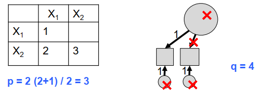
Example of under-identified model (df < 0): 1 factor, 2 items

• quantity of information to estimate the model: \(p = \frac{n(n+1)}{2} = \frac{2(2+1)}{2}=3\)
• number of unique parameters: 5 (1 factor variance, 2 loadings, 2 residual variances).
• 1 fixed loading (marker method)
• 4 free parameters (5 unique - 1 fixed)
• degrees of freedom: 3-4=-1 (under-identified)

Note

Rules of identification:

• every factor has been assigned a metric
• there are at least 3 indicators in 1-factor model and at least 2 indicators in multifactor models

5 Fit-indices/Fit-measures for CFA

5.1 Model quality

Exactly one solution is possible for exactly identified models, several solutions are possible for over-identified models, the best solution must be found.

The examination at model level (overall model) suggests to check whether the empirical variance-covariance matrix is reproduced as well as possible by the model-theoretical variance-covariance matrix.

Traditionally, we use the Chi-Square Test:

• H0: empirical covariance matrix = model-theoretical covariance matrix
• Chi-Square value is not meaningful by itself: the smaller the better
• In just-identified models, Chi-Square is always 0, but it means that we simply cannot estimate the model fit.
• Chi-Square is sensitive to sample size (it is always large and significant, when N>1,000).
• Chi-square is obtained from the Maximum Likelihood statistic.

5.2 Approximate fit indexes

To resolve the problem related to the Chi-square sensitivity under large samples, approximate fit indexes that are not based on accepting or rejecting the null hypothesis were developed.

These approximate fit indexes can be classified into incremental and absolute fit indexes.

• Incremental fit indexes: assesses the ratio of the deviation of the user model from the baseline model (worst model) against the deviation of the saturated model (best fitting model) from the baseline model.
  • Recommended values: >0.90 or >0.95.
  • CFI (Comparative Fit Index)
  • TLI (Tucker-Lewis Index)
• Absolute fit indexes: compare the user model to the observed data.
  • Recommended values: <0.08
  • RMSEA (Root Mean Squared Error of Approximation)

5.3 Comparison of different models

Comparing different models can be useful when we have competing theoretical models:

• lower RMSEA = descriptively better model
• larger CFI = descriptively better model

Note

Statistically verified comparisons between competing models only possible with nested models (= models are exactly identical except that one path is more/less estimated):

• one- and two-factor models (but not 2- and 3- or more factors)
• correlated and non-correlated factors
• with residual covariance and without it

To do so, we can rely on the Chi-Square Difference Test. If the test is not significant, then the model with more fixed parameters (i.e. the more economical and therefore theoretically clearer model) is no worse than the model in which more paths are allowed.

5.4 CFA example: Schulz et al. (2018)

6 Quiz

6.1 How to identify a 1-factor 2-items model?

When there are only two items, you have 2(2+1)/2=3 elements in the variance covariance matrix. However, there are 5 free parameters (2 residual variances, 2 loadings and 1 factor variance). Even if we used the marker method, which the default, that leaves us with 1 less parameter, resulting in 4 free parameters when we only have 3 to work with.

Solution

Use the variance standardization method and equate the second loading to equal the first loading.

#one factor, two items (var std)
m <- 'f1 =~ a*q1 + a*q2' 
onefac2items <- cfa(m, data=dat, std.lv=TRUE) 

6.2 Do the marker and the variance stand. method give the same results?

e.g. 1-factor, 3-items model

With 3-items, we have 3(3+1)/2=6 elements in the variance-covariance matrix. There are 7 free parameters (3 residual variances, 3 loadings and 1 factor variance).

Solution

Marker method: it leaves us with 1 less parameter (1 of the loadings), resulting in 6 free parameters. Therefore, the degrees of freedom is 6-6=0.

Variance standardization method: we fix 1 factor variance. That leaves us with 1 less parameter, resulting in 6 free parameters. Therefore, the degrees of freedom is 6-6=0.

6.3 What if we include the intercepts?

#one factor three items, with means
m  <- ' f  =~ q1 + q2 + q3
          q1 ~ 1
          q2 ~ 1
          q3 ~ 1'
onefac3items_n <- cfa(m, data=dat)

Solution

p = n(n+1)/2 + n = 3(3+1)/2+3=9

Total number of parameters: 3 intercepts, 3 loadings, 1 factor variance and 3 residual variances, thus 10.

Variance standardization method: we fix the factor variance to 1.

Free parameters: 10 unique parameters - 1 fixed parameters, thus 9.

Degrees of freedom: 9 known values - 9 free parameters. Therefore, our degrees of freedom is 0 and we have a just-identified model.

Conclusion: adding in intercepts does not actually change the degrees of freedom of the model.