15 Longitudinal data analysis
15.1 Longitudial data analysis with panel data
A panel is usually denoted by having multiple entries (rows) for the same entity (e.g. respondent, company, etc) in a dataset. The multiple entries are due to different time periods at which the entity was observed.
15.2 The problem with OLS
OLS can be used to pool observations of the same entity recorded at different time points. However, observations of the same entity are then treated as if they originate from other entities. Important influences like serial correlation of observations within the same entity cannot be considered, leading to biased estimates.
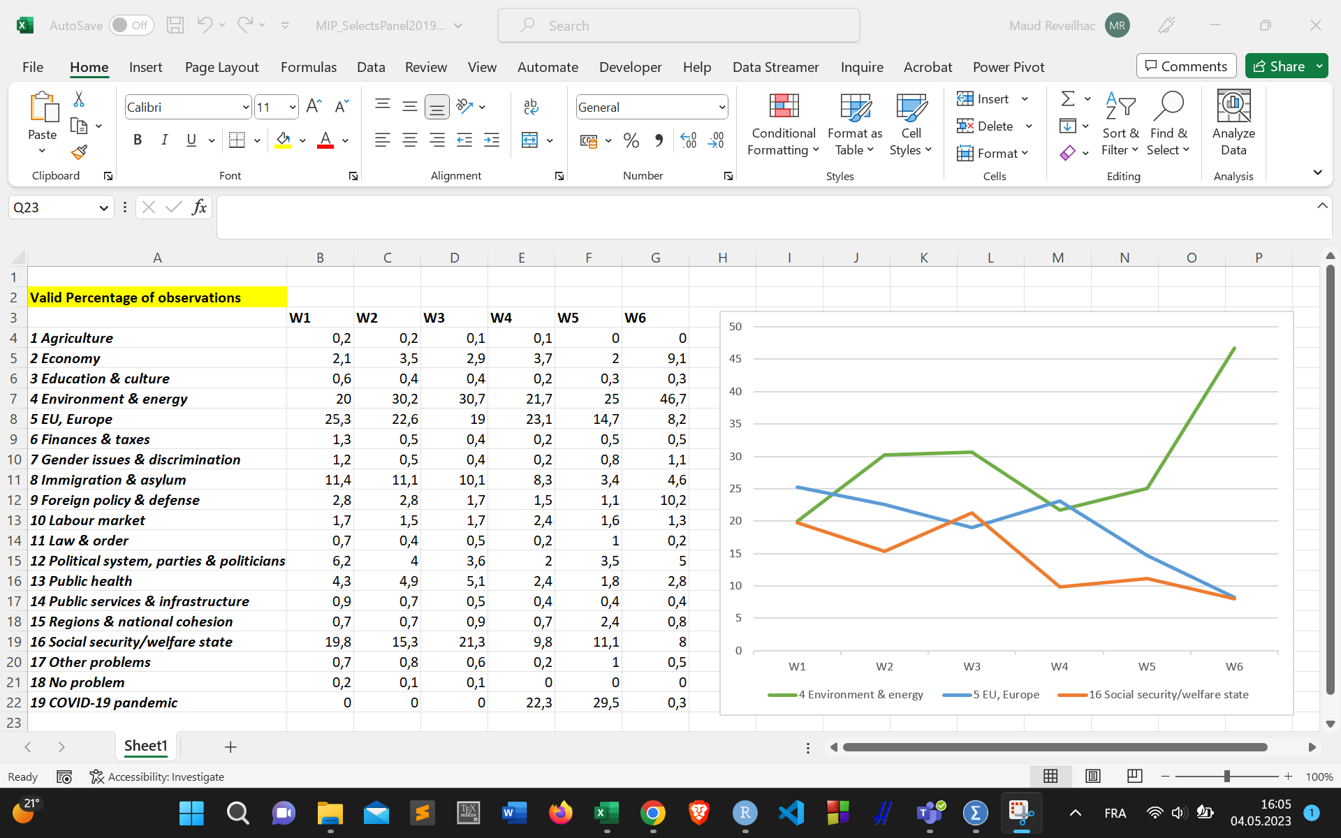
For instance, we might be interested in knowing what factors affect people’s change in their opinion about what is the most important problem facing the country. The next figure displays the change in the proportion of citizens’ concerns about the most important policy issues during the Swiss 2019 federal election campaign.
15.3 Fixed effect model
Fixed effect models (e.g., including time dummy variables) are sometimes applied to remove omitted variable bias. By estimating changes within a specific group (over time) all time-invariant differences between entities are controlled for.
The assumption behind the fixed effect model is that something influences the independent variables and one needs to control for it. The model removes characteristics that do not change over time, leading to unbiased estimates of the remaining independent variables on the dependent variable. Hence, if unobserved characteristics do not change over time, each change in the dependent variable must be due to influences not related to the fixed effects, which are controlled for.
Note that the influence of time-invariant independent variables on the dependent variable cannot be examined with a fixed effect model. In this case, Generalized Estimating Equation (GEE) models are more suitable for estimating a nonvarying (or average) coefficient in the presence of clustering.
GEEs are based on the quasi-likelihood theory and no assumption is made about the distribution of response observations (Liang and Zeger, 1986).
Furthermore, with GEEs, there is no need to make hypotheses on the structure of residuals compared to other models. This makes it possible to manage the panel data with a dichotomous dependent variable.
15.4 Multilevel model
Random effect models (with random intercept and/or slope) assume that any variation between entities is random and not correlated with the independent variables used in the estimation model. This also means that time-invariant variables (like a person’s gender) can be taken into account as independent variables. The entity’s error term (unobserved heterogeneity) is hence not correlated with the independent variables.
A decision between a fixed and random effects model can be made with the Hausman test assessing whether the individual error terms are correlated with the independent variables. The null hypothesis states that there is no such correlation (thus, one should go with a random effect model).The alternative hypothesis is that a correlation exists (thus, one should opt for a fixed effect model). The test is implemented in function phtest().
15.5 plm package
A useful ressource to conduct longitudinal data analysis is the plm R package. For more information about the plm package, refer to the following article:
Croissant, Y., & Millo, G. (2008). Panel Data Econometrics in R: The plm Package. Journal of Statistical Software, 27(2), 1-43. Available here
15.6 Analytical steps
As with MLM, we can start by conducting a fixed effect model by including dummy variables (e.g. for years). Then, the function pFtest() tests for fixed effects with the null hypothesis that pooled linear model is better than fixed effects.
In contrast to the fixed effect model, the random effect model assumes that an individual (entity) specific effect is not correlated with the independent variables. A decision between a fixed and random effects model can be made with the Hausman test. The null hypothesis states that there is no such correlation (thus, one should prefer the random effect model). The alternative hypothesis is that a correlation exists (thus, one should go for the fixed effect model).
The Breusch-Pagan Lagrange multiplier Test further helps to decide between a random effects model and a simple linear regression. This test is implemented in function plmtest() with the null hypothesis that the variance across entities is zero (thus, this means that there is no panel effect).
15.7 Heteroskedasticity and serial correlation
Testing for the presence of heteroskedasticity can be implemented in the function bptest().
For long time-series, a test for serial correlation of the residuals should be performed because serial correlation can lead to an underestimation of standard errors (too small) and an overestimation of R2 (too large). The test is implemented in function pbgtest() with the null hypothesis that there is no serial correlation.
In order to solve the issue of serial correlation, clustered standard errors have to be used. Clustered standard errors estimate the variance of the coefficient when independent variables are correlated within the entity. Correcting the standard errors can be done with the function vcovHC().
15.8 How it works in R?
See the lecture slides on longitudinal data analysis:
