Show the code
# load the data
library(foreign)
db <- read.spss(file=paste0(getwd(),
                "/data/protest.sav"),
                use.value.labels = F,
to.data.frame = T)Moderation analysis allows us to test for the influence of a third variable, Z, on the relationship between variables X and Y. Rather than testing a causal link between these other variables, moderation tests for when or under what conditions an effect occurs.
For instance, we can start with a bivariate relationship between an input variable X (e.g. training) and an outcome variable Y (e.g. test score). We can hypothesize that there is a relationship between them. A moderator variable Z (e.g. gender) is a variable that alters the strength of the relationship between X and Y.
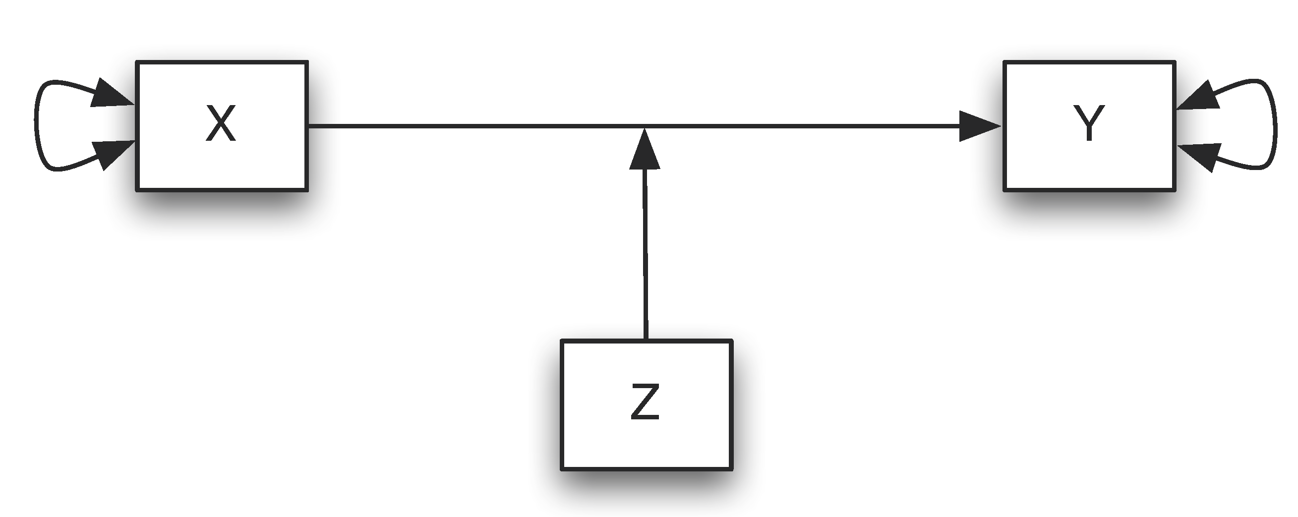
Moderators can strengthen, weaken, or reverse the nature of a relationship. Moderation can be tested by looking for significant interactions between the moderating variable (Z) and the independent variable (X).
Nota bene: Moderators (when) are conceptually different from mediators (how/why) but some variables may be a moderator or a mediator depending on your question.
The moderation is an interaction and therefore comparable to the interaction in ANOVA. If X and moderator are dichotomous, the moderation corresponds to a 2x2 ANOVA.
However, a moderator moderates the causal relationship from X to Y. The scale level can be dichotomous, categorical or metric. Furthermore, a moderator must be causally independent of X.
Technically, moderations (interactions) are linked multiplicatively in the regression analysis: A x B.
Statistically, the moderator and X must always be considered “in isolation” (not just as moderation or interaction).
An illustration of the similarity between a simple moderation analysis and a 2x2 ANOVA can be found below (this example is taken from Igartua and Hayes (2021)):
Moderation analysis can be conducted by adding one (or multiple) interaction terms in a regression analysis. For example, if Z is a moderator for the relation between X and Y, we can fit a regression model:
\[ Y = \beta_{0} + \beta_{1}*X + \beta_{2}*Z + \beta_{3}*XZ + \epsilon \]
\[ Y = \beta_{0} + \beta_{2}*Z + (\beta_{1} + \beta_{3}*Z)*X + \epsilon \] Thus, if \(\beta_{3}\) is not equal to 0, the relationship between X and Y depends on the value of Z, which indicates a moderation effect.
If Z is a dichotomous/binary variable (e.g. gender) the above equation can be written as:
\[ \beta_{0} + \beta_{1}*X + \epsilon \] for male (Z=0)
\[ \beta_{0} + \beta_{2} + (\beta_{1} + \beta_{3})*X + \epsilon \] for female (Z=1)
If X and/or moderator become significant, main effects are present. If the moderation term becomes significant, there is a moderation effect. The (possibly significant) influences of X and the moderator are then so-called “conditional” effects.
The value 0 usually has no meaningful meaning (e.g. in rating scales 1 to 5 there is no zero at all). Therefore, it is a good practice to centering means subtracting the overall mean from each value. The centering changes the interpretation decisively:
The change in meaning must be taken into account in the interpretation:
The moderation term is formed with moderator and X. However, the moderator and X are also contained individually in the regression equation. This often leads to multicollinearity (i.e. low tolerances or high VIF values).
If moderator and X are centered, the symptoms of multicollinearity are superficially defused. However, the multicollinearity itself remains.
Reminder: Multicollinearity means that predictors are (too strongly) related to each other. Since the moderation term also consists of A (or B), it can easily correlate with A (or B).
When the moderation effect becomes significant, it needs to be “illustrated” in order to make it interpretable. To do so, we can rely on simple slope analysis: comparison of the regression lines for low, medium and high levels of the moderator.
Typically, we use the mean value of the moderator, as well as the values + and - 1 SD are used, but theoretically any values can be considered.

This method suggests to conduct comparison of the regression equation for many characteristics of the moderator to identify areas of significance.
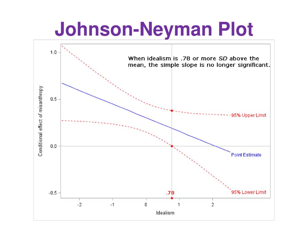
It is more useful than simple slopes for metric moderators, since illustrations result in less loss of information in the moderator’s levels. The effect (b) of the X on Y is now illustrated in the diagram as a function of the moderator (not to be confused with a regression line!), as well as the confidence interval for this effect:
A moderation analysis typically consists of the following steps:
A conceptual representation of a simple moderation model with a single moderating variable Z modifying the relationship between X and Y.
Let’s assume that X and Z are either dichotomous or continuous and the outcome variable Y is a continuous dimension suitable for analysis with linear regression, we have the following equations:
\[ \hat{Y} = a + b_1*X + b_2*Z + b_3*XZ = a + (b_1+b_3*Z)X + b_2*Z\] In this representation, the weight for X is not a single number but, rather, a function of Z: \(b_1+b_3*Z\). The output is sometimes called the simple slope of X or the conditional effect of X. The coefficients \(b_1\) and \(b_2\) may or may not have a substantive interpretation, depending on how X and Z are coded or, in the case of dichotomous X and Z, what two numbers are used to represent the groups in the data.
Important remarks:
Correct interpretation:
The following must be observed to report moderation analysis:
For a long time the PROCESS macro has been one of the best ways of testing moderations (interactions) when using SPSS. In December 2020, Hayes has released the PROCESS function for R.
To download Hayes’ PROCESS macro for R go here.
A tutorial about how to use the process() function in R can be found here.
A moderation analysis is a regression analysis in which the dependent variable (Y) is predicted from an independent variable (X) and a moderator (Z) and the interaction of both (XZ).
X and Z should be centered prior to analysis. On the one hand, this simplifies the interpretation of the results and, on the other hand, helps against the effects of multicollinearity in the model.
If the interaction term becomes significant, there is moderation.
The moderation effect can be illustrated by simple slopes and significance areas according to Johnson-Neyman.
See the lecture slides on moderation analysis:
The following article relies explains moderation (and mediation) analysis with an illustrative example:
Igartua, J. J., & Hayes, A. F. (2021). Mediation, moderation, and conditional process analysis: Concepts, computations, and some common confusions. The Spanish Journal of Psychology, 24, e49. Available here.
Please reflect on the following questions:
Simple moderation analysis is conceptually similar to a 2×2 ANOVA because both examine interactions between two variables to see whether the effect of one predictor on the outcome changes depending on another variable. In a 2×2 ANOVA, one tests whether the difference between group means on one factor varies across levels of another factor, which parallels how moderation tests whether the slope of a continuous predictor differs across levels of a moderator.
Main effects models focus on the independent influence of each variable while averaging over the levels of other predictors, assuming the effects are consistent across all conditions. In contrast, simple effects models break down the interaction by examining how one predictor affects the outcome at specific values or levels of the moderator, providing a more detailed understanding of where and how the interaction occurs.
The Johnson–Neyman technique improves upon the traditional simple slopes approach by identifying the precise regions of the moderator variable where the effect of the predictor is statistically significant. Instead of testing arbitrary low, medium, or high values, it provides a continuous range that shows where the predictor’s effect transitions from nonsignificant to significant, giving a clearer and more accurate picture of the conditional relationship.
Regression analysis is ultimately much more general and versatile because a regression approach does not require that the two variables being crossed be categorical. They can be categorical, continuous, or any combination of categorical and continuous.
No, as it is calculated by adding both coefficients from main effects + the interaction effect (51.545–4.446–4.535+12.555=55.119), but remember that the main effects are not significant
Lack of significant main effects does not prevent interpreting a significant interaction. Interactions test a different hypothesis (that the effect of X depends on W), and it’s common to see meaningful interactions with null main effects.
Proper way to proceed:
| True | False | Statement |
|---|---|---|
| Moderation analysis can be conducted by adding an interaction term in a regression analysis. | ||
| Moderation occurs when a third variable (Z) affects the relation between an independent variable (X) and the dependent variable (Y). | ||
| The simple (conditional) effect is the effect of X (or Z) on Y when Z (or X) is equal to 0. | ||
| Standardization of the variables is useful to mitigate multicollinearity. |
You can download the PDF of the exercises here: 
In this exercise, we will use the data “protest.sav” (Hayes, 2022) which can be downloaded  or here under “data files and code”. Especially, we will focus on the following variables:
We want to test the assumption that when women believe that sexism is a problem in society, they like the lawyer more when he protests sexism than when he doesn’t protest.
Start by drawing the regression equations.
The regression equation go as:
\[ Y_i = \beta_0 + \beta_1*Protest_i + \beta_2*Sexismus_i + \beta_3*(Protest*Sexismus_i) + \epsilon \]
Now, we want to know if the overall model is significant? Start by importing the data:
# load the data
library(foreign)
db <- read.spss(file=paste0(getwd(),
"/data/protest.sav"),
use.value.labels = F,
to.data.frame = T)Note that there are several ways to center the variables when creating the interaction term.
# interaction term
# without centering
db$ProtestXSexism1 = db$protest*db$sexism
# with centering
db$ProtestXSexism2 = (db$protest-mean(db$protest)) * (db$sexism-mean(db$sexism))
# z-standardization
# db$ProtestXSexism3 = scale(db$protest)*scale(db$sexism)
# view
head(db)
##   sexism liking respappr protest x Sexism_h_t ProtestXSexism1 ProtestXSexism2
## 1   4.25   4.50     5.75       0 4          1               0       0.5914260
## 2   4.62   6.83     5.75       0 6          1               0       0.3390229
## 3   4.62   4.83     5.25       0 4          1               0       0.3390229
## 4   4.37   4.83     4.25       0 5          1               0       0.5095655
## 5   4.25   5.50     2.50       0 3          1               0       0.5914260
## 6   4.00   6.83     4.75       0 3          1               0       0.7619686
Now, run the regression model:
# regression model (with centering)
m.cent = lm(liking ~ protest + sexism + ProtestXSexism2, data=db)
summary(m.cent)
##
## Call:
## lm(formula = liking ~ protest + sexism + ProtestXSexism2, data = db)
##
## Residuals:
##     Min      1Q  Median      3Q     Max
## -3.9894 -0.6381  0.0478  0.7404  2.3650
##
## Coefficients:
##                 Estimate Std. Error t value Pr(>|t|)
## (Intercept)      4.79659    0.58679   8.174 2.83e-13 ***
## protest          0.49262    0.18722   2.631  0.00958 **
## sexism           0.09613    0.11169   0.861  0.39102
## ProtestXSexism2  0.83355    0.24356   3.422  0.00084 ***
## ---
## Signif. codes:  0 '***' 0.001 '**' 0.01 '*' 0.05 '.' 0.1 ' ' 1
##
## Residual standard error: 0.9888 on 125 degrees of freedom
## Multiple R-squared:  0.1335, Adjusted R-squared:  0.1127
## F-statistic: 6.419 on 3 and 125 DF,  p-value: 0.0004439

# regression model (without centering)
m.roh = lm(liking ~ protest + sexism + ProtestXSexism1, data=db)
summary(m.roh)
##
## Call:
## lm(formula = liking ~ protest + sexism + ProtestXSexism1, data = db)
##
## Residuals:
##     Min      1Q  Median      3Q     Max
## -3.9894 -0.6381  0.0478  0.7404  2.3650
##
## Coefficients:
##                 Estimate Std. Error t value Pr(>|t|)
## (Intercept)       7.7062     1.0449   7.375 1.99e-11 ***
## protest          -3.7727     1.2541  -3.008  0.00318 **
## sexism           -0.4725     0.2038  -2.318  0.02205 *
## ProtestXSexism1   0.8336     0.2436   3.422  0.00084 ***
## ---
## Signif. codes:  0 '***' 0.001 '**' 0.01 '*' 0.05 '.' 0.1 ' ' 1
##
## Residual standard error: 0.9888 on 125 degrees of freedom
## Multiple R-squared:  0.1335, Adjusted R-squared:  0.1127
## F-statistic: 6.419 on 3 and 125 DF,  p-value: 0.0004439
How much variance does the model explain? Are there main effects or conditional effects? If yes, what do they look like?
The overall model is significant (p < .001) and explains 13.3% of the variance. We are allowed to interpret the results of the regression.
There is a significant conditional effect of protest when sexism = 0. It is not a main effect since interaction is also included.
Protest has an effect on the assessment if the moderator (sexism) has the value zero (= a medium level, since mean centered)
Is there a moderation effect?
# run the model without the interaction term
m0 = lm(liking ~ protest + sexism, data=db)
# compare the R2
summary(m.cent)$r.squared - summary(m0)$r.squared
## [1] 0.08119242
# get EtaSq
DescTools::EtaSq(m.cent)
##                      eta.sq eta.sq.part
## protest         0.047991546 0.052478399
## sexism          0.005136019 0.005892326
## ProtestXSexism2 0.081192415 0.085672955
If so, how much variance does this explain and what does this effect mean in general?
The interaction of protest and sexism perception is significant. There is a moderation effect.
The effect of the protest on the lawyer’s assessment varies depending on how strongly the subjects perceive sexism as a problem.
The interaction contributes 8.1% to explaining the variance. The dependent variable is thus better explained if moderation is taken into account.
Main effects are conditional effects when an interaction is present. After centering, you are testing the effect of each predictor at the mean of the other. So, the nonsignificant sexism coefficient simply means: Among participants at an average level of sexism belief, and when the lawyer does not protest, sexism does not significantly predict liking. That does not contradict the significant interaction — it just says the average effect is not strong on its own. So, the loss of significance after centering does not mean sexism stopped mattering. It means the interpretation of the coefficient changed: from an artificial reference (sexism = 0) to a meaningful one (sexism = average).
Illustrate the moderation effect graphically and interpret it. First, we can create an interaction plot:
# extract the needed coefficients
intercept.p0 = coefficients(m.roh)[1]
intercept.p1 = coefficients(m.roh)[1] + coefficients(m.roh)[2]
slope.p0 = coefficients(m.roh)[3]
slope.p1 = coefficients(m.roh)[3] + coefficients(m.roh)[4]
# interaction plot
par(mfrow=c(1,1))
farben = c("red","blue")
plot(db$sexism, db$liking, main="Interaction",
     col=farben[db$protest+1],pch=16,
     xlab="Sexism",ylab="Liking")
abline(intercept.p0,slope.p0,col="red")
abline(intercept.p1,slope.p1,col="blue")
legend("bottomleft",
       c("Protest=0","Protest=1"),
       col=c("red","blue"),pch=16)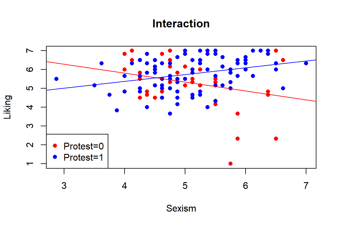
The code is computing the simple regression lines (simple intercepts and slopes) for each level of the binary moderator protest (0 vs 1) from the uncentered model m.roh:
\[ liking = \beta_0 + \beta_1(protest) + \beta_2(sexism) + \beta_3(protest * sexism) \] With protest coded 0/1, for protest = 0:
\[ liking = \beta_0 + \beta_2(sexism) \] \[ intercept.p0 = \beta_0 \] (line’s value at sexism = 0) \[ slope.p0 = \beta_2 \] (effect of sexism when protest = 0)
For protest = 1:
\[ liking = (\beta_0 + \beta_1) + (\beta_2 + \beta_3)sexism \] \[ intercept.p1 = \beta_0 + \beta_1 \] (baseline shift when protest = 1) \[ slope.p1 = \beta_2 + \beta_3 \] (effect of sexism when protest = 1)
Second, we can provide a Johnson-Neyman plot:
library(interactions)
m.simplified = lm(liking ~ protest*sexism, data=db)
johnson_neyman(m.simplified,"protest","sexism")
## JOHNSON-NEYMAN INTERVAL
##
## When sexism is OUTSIDE the interval [3.51, 4.98], the slope of protest is p < .05.
##
## Note: The range of observed values of sexism is [2.87, 7.00]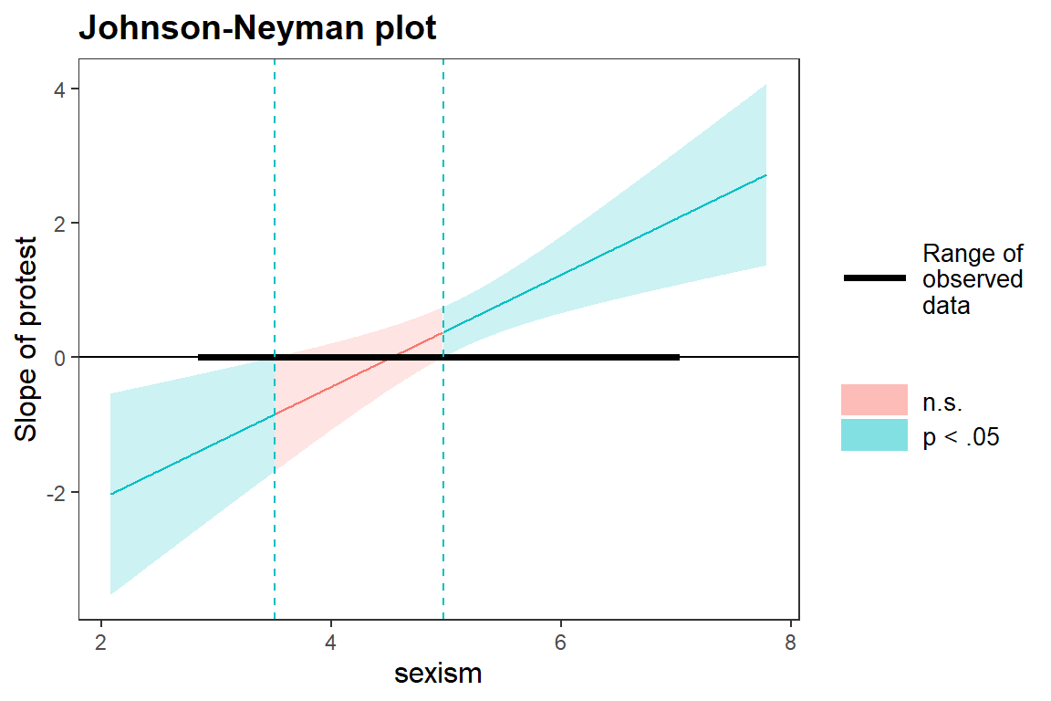
The Johnson–Neyman plot illustrates how the relationship between sexism and protest changes depending on the level of sexism. The horizontal black bar indicates the observed range of the data.
In short, sexism has no clear effect in the middle of the scale, but is negatively related to protest among individuals low in sexism, and positively related to protest among individuals high in sexism.
Now, divide the moderator into a dichotomous variable (sexism low vs. high) with a median split and recalculate the moderation analysis.
# Median split
db$sexism.ms = as.integer(db$sexism>=median(db$sexism))
What changes in the output?
# new model
m3 = lm(liking ~ protest*sexism.ms, data=db)
summary(m3)
##
## Call:
## lm(formula = liking ~ protest * sexism.ms, data = db)
##
## Residuals:
##     Min      1Q  Median      3Q     Max
## -3.9179 -0.6815  0.1263  0.7963  2.0821
##
## Coefficients:
##                   Estimate Std. Error t value Pr(>|t|)
## (Intercept)         5.6491     0.2125  26.584  < 2e-16 ***
## protest            -0.1154     0.2634  -0.438  0.66199
## sexism.ms          -0.7312     0.3122  -2.342  0.02074 *
## protest:sexism.ms   1.2090     0.3779   3.199  0.00175 **
## ---
## Signif. codes:  0 '***' 0.001 '**' 0.01 '*' 0.05 '.' 0.1 ' ' 1
##
## Residual standard error: 0.9967 on 125 degrees of freedom
## Multiple R-squared:  0.1195, Adjusted R-squared:  0.09839
## F-statistic: 5.656 on 3 and 125 DF,  p-value: 0.001148
# get EtaSq
DescTools::EtaSq(m3)
##                        eta.sq eta.sq.part
## protest           0.043987025 0.047581194
## sexism.ms         0.002000014 0.002266368
## protest:sexism.ms 0.072096985 0.075686621
# get the coeff
meanvalues = tapply(db$liking, list(db$protest,db$sexism.ms),FUN=mean)
meanvalues
##          0        1
## 0 5.649091 4.917895
## 1 5.533659 6.011489R-square significantly worse (probably due to loss of information during dichotomization) and the coefficients change slightly.
There are only two Simple Slopes because there are only two moderator levels. There are no Johnson-Neyman values.
Calculate the moderation analysis again with the variable «x» as the independent variable (it measure the lawyer protests to varying degrees on a scale of 1-7) and the metric moderator. What changes in the output?
# new model
m4 = lm(liking ~ x*sexism, data=db)
summary(m4)
##
## Call:
## lm(formula = liking ~ x * sexism, data = db)
##
## Residuals:
##     Min      1Q  Median      3Q     Max
## -4.0451 -0.6128  0.1029  0.7720  1.6583
##
## Coefficients:
##             Estimate Std. Error t value  Pr(>|t|)
## (Intercept)  8.65856    1.90366   4.548 0.0000126 ***
## x           -0.90210    0.45129  -1.999    0.0478 *
## sexism      -0.73604    0.36256  -2.030    0.0445 *
## x:sexism     0.21069    0.08563   2.460    0.0152 *
## ---
## Signif. codes:  0 '***' 0.001 '**' 0.01 '*' 0.05 '.' 0.1 ' ' 1
##
## Residual standard error: 1.009 on 125 degrees of freedom
## Multiple R-squared:  0.09858,    Adjusted R-squared:  0.07695
## F-statistic: 4.557 on 3 and 125 DF,  p-value: 0.004584
# get EtaSq
DescTools::EtaSq(m4)
##               eta.sq eta.sq.part
## x        0.046574596  0.04912969
## sexism   0.006844541  0.00753586
## x:sexism 0.043654300 0.04619148Now the hypothesis is that the more women believe that sexism is a problem, the more they like the lawyer, the more she protests.
The coefficients change, the explanation of variance overall and through the interaction alone is weaker in each case (but this is simply because it is a completely different and only a simulated variable).
What changes in the graphics?
# plots
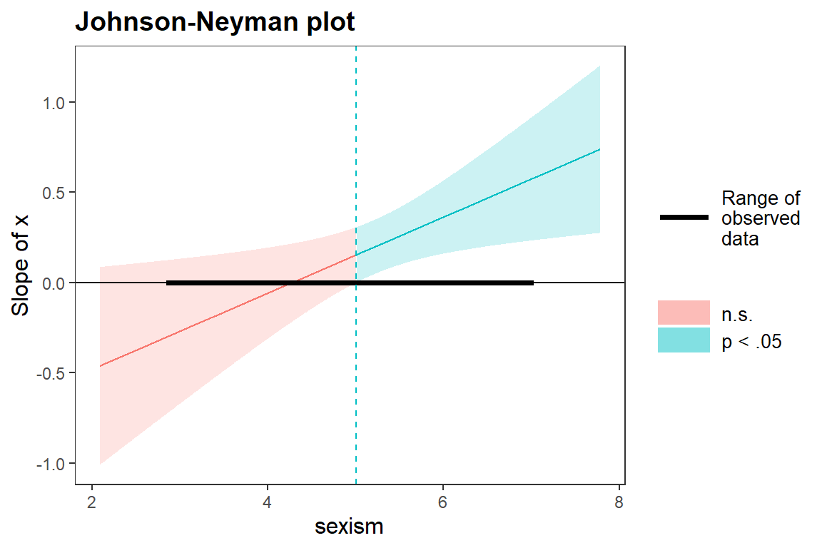
johnson_neyman(m4,"x","sexism")
## JOHNSON-NEYMAN INTERVAL
##
## When sexism is OUTSIDE the interval [0.20, 5.01], the slope of x is p < .05.
##
## Note: The range of observed values of sexism is [2.87, 7.00]