Logistic regression is a model with a binary dependent variable (e.g., 0 = not elected versus 1 = elected). In this case, we are interested in knowing the probability of a phenomenon (e.g., get elected, lose a job, becoming sick, etc) to occur:
\[Y(P=1)=a+bX+e\]
also referred as Linear Probability Model (LPM). However, the interpretation is complicated be that fact that applying LPM may return values outside the [0,1] interval (probabilities are necessary between 0 and 1!).
Example: An increase in political experience (e.g., number of years a candidate has joined his party) by 1 year increases/decreases the probability of being elected as a national representative by \(b*100\) percentage points.
Simple regression: professional consultant example
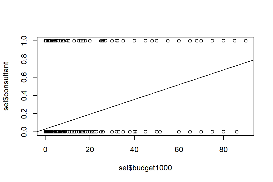
Let’s predict the probability that a candidate employs professional consultants explained by the available campaigning budget in a linear regression framework.
We can first look at the distribution of political candidates employing a consultant:
We see that the linear line is not ideal and does not fit the data. A dichotomous dependent variable does not display a normal distribution. It cannot have a linear relationship with an explanatory variable. Therefore, linear regression could make predictions smaller than 0 and bigger than 1, which is not possible!
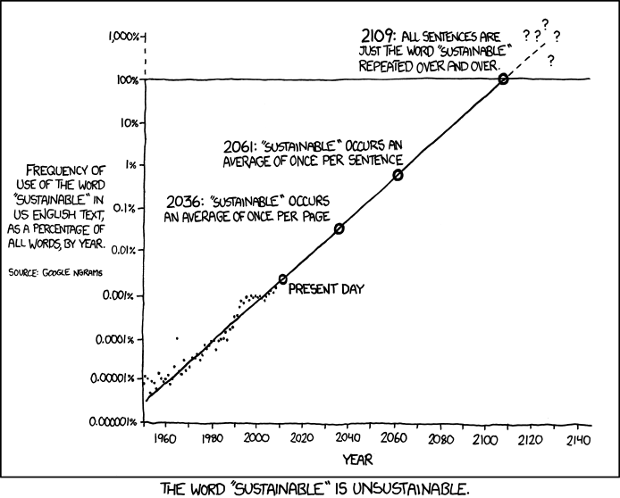
Example: We may observe that by 2109, the word “sustainable” will be used only in English-language publications if the model’s tendency is accurate. Therefore, even though a trend is evident in this case, the linear model does a less than ideal job of capturing it. Linear regression, which forecasts results on a scale from negative infinity to infinity, is no longer logical given that these categories are nominal. Rather, we require a tool that allows us to make categorical predictions.
6.2 The problem with LPM
LPM poses several issues:
non-linearity
non-normal distribution of the errors (only two possible outcomes)
heteroscedasticity
difficulty in interpreting the results
Therefore, we need a non-linear model predicting probability of an event which remains in [0,1] bounds. The question is how to constrain all possible outcomes between 0 and 1.
Non-linear probability models are essential in social sciences which often deal with categorical dependent variables (e.g., binary, ordinal, nominal). There exists several models depending of the measurement level of the dependent variable. Logistic regression allows to predict models for categorical dependent variables in the simplest binary form and is part of the Generalized Linear Model (GLM) framework:
Binomial: binary variable
Multinomial: categorical variable
Gaussian: interval variable
Poisson: count data (discrete)
Gamma: >0 (non-discrete)
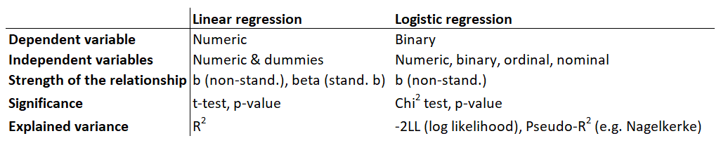
6.3 Differences between linear and logistic regressions
6.4 Odds ratio (OR)
OR is the relative chance of an event happening under two different conditions. In other words, it is the ratio of the odds of an event occurring in one group to the odds of it occurring in another group (relative odds).
Let’s take the following games:
Game 1: profit of 20, loss of 100, odds of 20/100=0.2
Game 2: profit of 10, loss of 100, odds of 10/100=0.1
Here, the OR is 0.2/0.1=2. Since the OR is >1, it suggests that the odds in game 1 is higher than in game 2: the relative chance of winning instead of loosing is 2-times higher in game 1.
OR: further examples
An OR of 1.3 means there is a 30% increase in the odds of an outcome.
An OR of 2 means there is a 100% increase in the odds of an outcome (same as saying that there is a doubling of the odds of the outcome).
An OR of 0.3 means there is an 70% decrease in the odds of an outcome.
6.5 Constraining all possible outcomes
6.5.1 Step 1: p to odds
First, we need to transform \(Y\) into \(p/(1-p)\) so that the binary dependent variable can be expressed as a function of continuous positive values ranging from 0 to \(+\infty\).
The formal interpretation suggests that “a unit increase in X changes the odds that Y=1 instead of Y=0 by a factor of \(e^z\) (antilog of the odds), all else equal.
OR less than 1= negative effect (negative log-odds)
OR greater than 1= positive effect (positive log-odds)
But, OR give no indication about the magnitude of the implied change in the probabilities. Let’s look at the following example of two societies:
Absolute differences versus odds ratio
In the above scenario, different differences in probabilities can be associated to the same odds ratio. The social mechanisms responsible for gender effect on having work are the same in the two societies, but the intensity of the effect resulting from those mechanisms is much stronger in A than B.
Note that OR can be expressed as % change in the odds \(100*(OR-1)\).
6.5.2 Step 2: odds to log odds
Up to now, we have \(odds=p/(1-p)\), which we now transform into log odds: \(ln(p/(1-p))\).
If p=0.5, odds=1 and log odds: 0, which suggests no effect
If p=0.8 of success (0.2 of failure), odds=4 and log odds: 1.38, which suggests a positive effect
If p=0.8 of failure (0.2 of success), odds=1/4 and log odds: -1.38, which suggests a negative effect
So, for log odds, only the sign (direction of the coefficient) can be interpreted.
6.5.3 Step 3: back to probabilities
The problem with log odds (also called logit) is that they are not easy to interpret: “logarithmic odds of an increase in budget by one franc on being elected”. Therefore, we need to transform log odds into probabilities:
\[P_i(y=1)=\frac{e^{a+b_1x_1+b_2x_2}}{1+e^{a+b_1x_1+b_2x_2}}\] where \(e^1=2.71828\) and \(e^{ln(x)}=x\).
Logistic transformations
Why do we need these three steps?
In logistic regression, the goal is to predict probabilities — values between 0 and 1. However, if we tried to model probability directly with a linear equation, the predicted values could easily fall below 0 or above 1, which makes no sense for probabilities. To fix that, we use a series of mathematical transformations that let us use a linear model while keeping probabilities valid.
From probabilities to odds: Probabilities are bounded between 0 and 1, but odds \((p / (1 – p))\) can take any positive value from 0 to infinity. Example: if p = 0.8, odds = 0.8 / 0.2 = 4. This step stretches probabilities into an unbounded scale (0 → inf.), which makes them easier to model mathematically.
From odds to log odds (the logit): Odds are still positive only but linear regression can handle both negative and positive numbers. So we take the natural log of the odds, which gives us log odds (logit). Example: if odds = 4, then log(4) ≈ 1.39; if odds = 0.25, then log(0.25) = –1.39. The logit can now range from –inf to +inf. The coefficients (\(β\)) can then be estimated using ordinary regression logic.
From log odds back to probabilities: After fitting the model, we do not want to stay in log-odds form because it is not intuitive to interpret. So we transform back to probabilities. This guarantees that the predicted values will always fall between 0 and 1.
6.6 Relationship between probability, logit and odds ratio
If p is a probability, then p/(1 − p) is the corresponding odds. Furthermore, the logit of the probability is the logarithm of the odds:
Relationship between probability, logit and odds ratio
6.7 Marginal predictions
The main benefit of marginal predictions is that it leaves everything at the mean, except for the variable that you are interested in. Therefore, one variable is changing while the others are not.
For a continuous covariate, the margins compute how P(Y=1) changes as X changes from 0 to 1, controlling for other variables in the model. For a dichotomous independent variable, the marginal effect equates the difference in the adjusted predictions for two groups (e.g., for women and men). For discrete covariate, the margins compute the effect of a discrete change of the covariate (discrete change effects).
6.8 Model fit
\(R^2\) in OLS is a measure for model fit. It is based on differences between real observations and the regression line. It tries to remove as much error as possible.
In logistic regression, there is no comparable measure since all values on Y are either 1 or 0 . We are explaining probabilities (not explained variance). The model fit is based on Maximum Likelihood Estimation (MLE) which tries to guess parameters that have highest likelihood of producing observed sample patterns. Likelihood is the probability that our statistical model is actually found in a sample, thus the better the model fits the data, the more likelier it is.
The smaller the Log likelihood the better the model fit: by how much Log likelihood has decreased by adding (a) variable(s), and by calculating the significance of this difference. It is possible to compare models statistically by a Chi-squared test.
Note 1: Pseudo \(R^2=(-2LL0 - -2LL1)/-2LL0\) has no clear interpretation, but provides a good way to compare models (rather than assessing fit).
Note 2: Akaike Information Criterion (AIC) and Bayesian Information Criterion (BIC) are alternative measures (the smaller AIC or BIC, the better the model fit).
6.9 In a nutshell
Logistic regression models the probability of a binary outcome, such as being elected (1) or not elected (0). It is used when the dependent variable is categorical, typically binary.
A simple linear regression model is not appropriate in this case because it can produce predicted values outside the range of 0 and 1. It violates key assumptions such as linearity, normality of errors, and homoscedasticity.
Logistic regression solves this by using a nonlinear transformation that constrains predicted probabilities to stay within the 0–1 interval. It does this through the logit function, which expresses the log of the odds of the event occurring.
In logistic regression, the odds represent the ratio of the probability of success to the probability of failure \((p / (1 – p))\). The odds ratio (OR) compares these odds across groups. An OR greater than 1 indicates a positive effect, while an OR less than 1 indicates a negative effect. For example, an OR of 2 means the odds of success are twice as high in one group compared to another.
The logistic model involves three transformations: converting probabilities to odds, odds to log odds (logit), and log odds back to probabilities. A one-unit increase in X changes the odds of Y = 1 by a factor of \(e^{(β1)}\), holding all other variables constant.
Marginal effects are used to interpret results more intuitively. They show how the predicted probability of the event changes as one variable changes, keeping all other variables constant.
Model fit in logistic regression is assessed using Maximum Likelihood Estimation (MLE), which identifies the parameter values that make the observed data most likely. Fit statistics such as Log Likelihood, Akaike Information Criterion (AIC), and Bayesian Information Criterion (BIC) are used for model comparison, with lower values indicating better fit. Pseudo \(R^2\) values can be used to compare models.
6.10 How it works in R?
See the lecture slides on logistic regression:
You can also download the PDF of the slides here:
6.11 Quiz
True
False
Statement
Logistic regression is used to make predictions about a dichotomous dependent variable.
Odds can be defined as the number of times something occurs relative to the number of times it does not occur.
If the odds ratio of a dummy variable is greater than 1, then the group captured in the dummy variable is predicted to be more likely than the reference group to have something occur (a dummy variable is a binary variable coded as 0 or 1 to represent the absence or presence of a characteristic).
When there is exactly a 0.5 probability of something occurring, the log odds are 1.
My results will appear here
6.12 Example from the literature
The following article relies on logistic regression as a method of analysis:
Vogler, D., & Schäfer, M. S. (2020). Growing influence of university PR on science news coverage? A longitudinal automated content analysis of university media releases and newspaper coverage in Switzerland, 2003‒2017. International Journal of Communication, 14, 22. Available here.
Please reflect on the following questions:
What is the research question of the study?
What are the research hypotheses?
Is logistic regression an appropriate method of analysis to answer the research question?
Solution
When modeling whether a news item was based on a university media release (yes/no) or whether tone is positive vs. not, logistic regression is appropriate because it estimates the log-odds of a binary event. If your dependent variable is a count (e.g., number of overlaps/borrowed passages) or share (proportion of coverage based on releases), then Poisson/negative binomial or fractional logit/beta regression would be more appropriate.
What are the main findings of the logistic regression analysis?
And some more questions from the tutors:
How do you approach reading long regression tables in articles (without relying on the surrounding text and interpretation)? What could be typical interpretative steps?
Solution
We can ask ourself the following questions when interpreting a table:
What does the table show, i.e., what is in the title, footnotes, rows and columns?
What is the dependent variable, what are the independent and control variables, what are the reference categories?
What method was used?
What do the coefficients listed in the table represent and what do their signs and sizes show?
Where do you see significance levels?
Start interpreting line by line then connect to the hypotheses/research question(s)
How do you interpret Odds Ratio?
Solution
Odds ratio indicates how the odds of Y=1 change with a unit increase in X. A unit increase in X changes the odds that Y=1 instead of Y=0 by a factor of \(e^z\) (antilog of the odds), holding all else equal. OR < 1 = negative effect, OR > 1 = positive effect meaning it only shows direction and strength of effect, not the magnitude of change in probabilities.
Take a look at the PR influence coefficient (3.19**) in Table 1. What does it mean for our analysis?
Solution
The odds ratio of tone in the media article being positive when there is press release influence on the article is 3.19. It means that the positive tone of the article is predicted to be there much more likely than not to be there, when there is influence of the press release on the article. In other words, if there is PR influence, the tone will more likely be positive than not positive.
6.13 Time to practice on your own
You can download the PDF of the exercises here:
6.13.1 Exercise 1: probability of hiring a consultant according to campaign personalization
For instance, we are interested in measuring the likelihood of hiring a consultant (Y) explained by personalized style of campaigning (X). To do so, we will rely on the data covering the Swiss part of the Comparative Candidate Survey. We will be using the Selects 2019 Candidate Survey.
We can look at the likelihood of hiring of consultant (B11) by the level of campaign personalization (where B6 is recoded as 0=attention to the party and 10=attention to the candidate):
Now, we can calculate the odds of hiring a consultant for a very personalized campaign (personalization = 10):
Interpretation
\[\frac{0.17}{(1-0.17)} = 0.2 \] This suggests that for each candidate without a consultant, there are 0.2 candidates hiring a consultant. Alternatively:
\[\frac{(1-0.17)}{(1-(1-0.17))} = 4.9 \] This suggests that for each candidate hiring a consultant, there are 4.9 candidates without a consultant.
Now, calculate the odds of hiring a consultant for a very low personalized campaign (personalization = 0):
Interpretation
\[\frac{0.03}{(1-0.03)} = 0.03 \] Therefore, the odds ratio is: 0.2/0.03 = 6.7, suggesting that the odds of hiring a consultant are 6.7 higher for candidates with a very high personalized campaign than candidates with a very low personalized campaign.
The logit of the dependent variable (Y) is estimated by the following equation:
The logit does not indicate the probability that an event occurs. Apply the necessary transformation to know this probability (prob(Y=1)):
Answer
\[ proba = \frac{exp^{logit}}{1+exp^{logit}} \]
Let’s go back to our example and run the logistic regression:
Show the code
model2 <-glm(consultant ~ personalization, data=sel, family="binomial")summary(model2)## ## Call:## glm(formula = consultant ~ personalization, family = "binomial", ## data = sel)## ## Coefficients:## Estimate Std. Error z value Pr(>|z|) ## (Intercept) -3.54005 0.19321 -18.32 < 2e-16 ***## personalization 0.22052 0.03132 7.04 1.92e-12 ***## ---## Signif. codes: 0 '***' 0.001 '**' 0.01 '*' 0.05 '.' 0.1 ' ' 1## ## (Dispersion parameter for binomial family taken to be 1)## ## Null deviance: 1007.64 on 1854 degrees of freedom## Residual deviance: 957.86 on 1853 degrees of freedom## AIC: 961.86## ## Number of Fisher Scoring iterations: 5
Coefficients in the above output are log odds: 0.22 means that by augmenting the personalization of one point, log odds change by 0.22.
Now, assess the odds of hiring a consultant for a very personalized campaign (personalization=10):
Interpretation
The odds ratio for the personalization variable is exp(0.22)=1.24. This suggests that, for each unit increase on the personalization scale, the odds increase by a factor of 1.24, which is equivalent to an increase of 24%.
Beware that the odds ratio does not provide information about the probability of hiring a consultant. We can calculate the probability as follows:
\[ Logit = -3.54 + 0.22*10 = -1.34 \]
\[ Probability = \frac{exp(logit)}{1+exp(logit)} = \frac{e^{-1.34}}{(1+e^{-1.34})} = 0.79 \]
6.13.2 Exercise 2: predict the reliance of social media as campaigning tool
Using the same dataset, let’s investigate the following question: how does the level of campaign personalization and the fact of being affiliated to a governmental party, and being an incumbent affect the reliance of social media as campaigning tool?
In this scenario, the binary outcome is whether politicians rely on social media (combination of B4m and B4p) and the predictors are personalization (B6), being affiliated to a governmental party (based on T9), and being an incumbent (T11c).
Let’s prepare the data, including the selection and recoding of the relevant variables:
Now, we can conduct logistic regression and interpret the findings. Recall that, for log odds, we interpret only the sign of the coefficients (positive/negative). Coefficients smaller than 0 suggests a negative effect (negative log odds) and coefficients larger than 0 suggest positive effect (positive log odds). You can also transform to percentages using the formula 100*(OR-1):
Show the code
mod <-glm(SMuse ~ personalization + in_gov + incumbentNC, data=sel, family ="binomial")summary(mod)## ## Call:## glm(formula = SMuse ~ personalization + in_gov + incumbentNC, ## family = "binomial", data = sel)## ## Coefficients:## Estimate Std. Error z value Pr(>|z|) ## (Intercept) 0.26890 0.08100 3.320 0.000901 ***## personalization 0.16152 0.02046 7.896 2.89e-15 ***## in_gov1 0.08618 0.09972 0.864 0.387475 ## incumbentNC1 0.96787 0.30413 3.182 0.001461 ** ## ---## Signif. codes: 0 '***' 0.001 '**' 0.01 '*' 0.05 '.' 0.1 ' ' 1## ## (Dispersion parameter for binomial family taken to be 1)## ## Null deviance: 2585.2 on 2094 degrees of freedom## Residual deviance: 2487.0 on 2091 degrees of freedom## AIC: 2495## ## Number of Fisher Scoring iterations: 4# transformationexp(coef(mod))## (Intercept) personalization in_gov1 incumbentNC1 ## 1.308526 1.175299 1.090003 2.632324
Interpretation
The logistic regression model examined how personalization, governmental party affiliation, and incumbency affect politicians’ reliance on social media as a campaigning tool.
The results show that both personalization and incumbency have positive and statistically significant effects, while being affiliated with a governmental party does not.
Specifically, for each one-unit increase in personalization, the odds of relying on social media increase by about 17 percent (100(1.17-1)), controlling for the other factors. Incumbents are about 2.6 times more likely to rely on social media than non-incumbents, corresponding to roughly a 163 percent increase in odds.
The marginal effects indicate a change in predicted probability as X increases by 1. For categorical predictors, you have to take the predicted probability of the group A minus the predicted probability of the group B.
There are different ways of calculating predicted probabilities. In the social sciences, the most commonly used are Adjusted Predictions at the Means (APMs). For instance, we can assess the predicted probabilities of using social media for political incumbents, when the personalization level is at the mean and for incumbent not affiliated to a party in government.
Nota bene: Marginal Effects at the Means (MEMs) are calculated by taking the difference of two APMs. Let’s also calculate the predicted probabilities of using social media for political non-incumbents, when the personalization level is at the mean and for politicians not affiliated to a party in government. Then, calculate the difference between both predicted probabilities:
Predicted probabilities indicate that, at the mean level of personalization and outside government, incumbents have an estimated probability of 0.89 of using social media, compared to 0.75 for non-incumbents, a difference of about 14 percentage points.
In logistic regressions, there is no such R-squared value for general linear models. Instead, we can calculate a metric known as McFadden’s R-Squared, which ranges from 0 to just under 1, with higher values indicating a better model fit. We use the following formula to calculate McFadden’s R-Squared:
The McFadden’s R-squared value of 0.038 suggests that the model has modest explanatory power, which is common for behavioral data of this type.
Overall, the findings imply that greater campaign personalization and incumbency significantly increase the likelihood of using social media as a campaigning tool, while party affiliation with the government does not exert a measurable influence.