4 ANOVA

4.1 What is ANOVA?

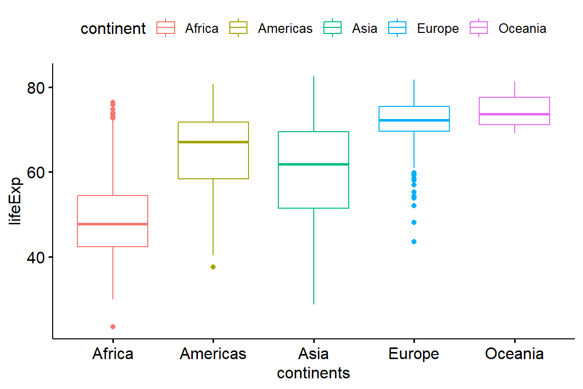
An ANOVA (Analysis of Variance) is used to determine whether or not there is a statistically significant difference between the means of three or more independent groups. The two most common types of ANOVA are the one-way ANOVA and two-way ANOVA.

The one-way analysis of variance (ANOVA), also known as one-factor ANOVA, is an extension of the independent two-sample t-test for comparing means when more than two groups are present. You can use the t-test if you just have two groups. The F-test and the t-test are equivalent in this scenario.

4.1.1 One-way and two-way ANOVA

One-way ANOVA is used to determine how one factor (or independent variable, IV) impacts a response variable (or dependent variable, DV).

Example: political affiliation impacts on media coverage.

Two-way ANOVA is used to determine how two factors impact a response variable, and to determine whether or not there is an interaction between the two factors on the response variable.

Example: political affiliation and gender impact on media coverage.

4.1.2 Regression versus variance analyses

Regression analysis:

Relationships between two variables
Metric independent variables
Logic: “The bigger X, the bigger Y”
Useful to evaluate survey data

Analysis of variance:

Differences between two or more groups
Categorical independent variables
Logic: “More in group A than in group B”
Useful for evaluating experimental data

But, both methods are based on the same principle, the general linear model and the F-test.

Regression: The quality of the model results from the deviation of the individual values from the regression line

ANOVA: Model quality results from the deviation of the individual values from the group mean

4.1.3 Basic hypotheses of ANOVA

The data is divided into several sub-groups using one single grouping variable (also called factor variable). The basic hypotheses for ANOVA tests are:

Null hypothesis: the means of the various groups are identical.
Alternative hypothesis: at least one sample mean differs from the rest.

ANOVA can only be used when the observations are gathered separately and randomly from the population described by the factor levels. That is, each factor level’s data has to be normally distributed and the variance in the sub-populations must be similar (this can be verified using Levene’s test).

4.1.4 T-test and F-test

If you want to compare the means of two groups, you can do a t-test.

If you want to compare the means of more than two groups, one would have to compare each group with each other. However, the alpha error cumulation arises as the error probability of 5% is reclaimed each time for pairwise comparisons: \[ \alpha = 1 - (1 - \alpha)n \]

where n is the number of tests.

The solution consists in using a test that checks whether at least 2 groups differ significantly from each other: F-test, which has no alpha-error accumulation.

4.1.5 Decomposition of the variance

To find the total amount of variation within our data we calculate the difference between each observed data point and the grand mean. We then square these differences and add them together to give us the total sum of squares (TSS, also called SST on the next figure).

\[ TSS = \sum{(\hat{y}_{ij} - \hat{y}_{Grand})^2} \] The model sum of squares (MSS, also called SSM on the next figure) requires us to calculate the differences between each participant’s predicted value and the grand mean: it is the sum of the squared distances between what the model predicts for each data point (i.e., the dotted horizontal line for the group to which the data point belongs) and the overall mean of the data (the solid horizontal line).

\[ MSS = \sum{n_j(\hat{y}_j - \hat{y}_{Grand})^2} \] The final sum of squares is the residual sum of squares (SSE, also called SSR on the next figure), which tells us how much of the variation cannot be explained by the model. The simplest way to calculate SSE is to subtract MSS from TSS. It is calculated by looking at the difference between the score obtained by a person and the mean of the group to which the person belongs. These distances between each data point and the group mean are squared and then added together to give the SSE.

\[ SSE = \sum{(y_{ij} - \hat{y}_i)^2} \]

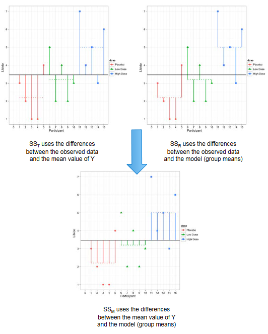
The original figure can be found here.

4.1.6 Mean Squares (MS)

The sum of squares depends on the number of groups and the number of cases per group. MS are variances calculated by dividing the SS by the corresponding number of degrees of freedom.

Model Mean Sum of Squares: \(MS_M = \frac{MSS}{df_M}\), \(df_M = k-1\).
Mean sum of squares of the residuals: \(MS_R = \frac{RSS}{df_R}\), \(df_R = k(n_j-1) = n-k\).

The test variable \(F_{Ratio}\) is calculated as follows: \(F = \frac{MS_M}{MS_R}\).

Note that n is the number of observations by group and k is the number of groups.

Calculate the F-statistics

Let’s assume that we have three groups to compare (A, B, and C). The following steps must be undertaken in one-way ANOVA:

Calculate the common variance, often known as residual variance or variance within samples: \(SS_w\)
Calculate the difference in sample means as follows:
- Calculate the average of each group
- Calculate the difference in sample means: \(SS_b\)

The F-statistic is calculated based on the ratio of \(SS_b/SS_w\). Note that a lower ratio suggests that the means of the samples being compared are not significantly different. A greater ratio, on the other hand, indicates that the differences in group means are significant.

The figure below shows the calculation of the F-statistic for one-way ANOVA offer. You can click on the figure to download the excel file.

4.1.7 Effect of two or more factors

To compare the influence of several different factors, it is necessary to test the interaction hypotheses: influence of a factor depending on one or more other factors (A and B).

\(MSS_A\): Calculation with the groups of the factor A (we pretend that B does not exist)
\(MSS_B\): Calculation with the groups of the factor B (we pretend that A does not exist)
\(MSS_{AB}\): \(MSS-MSS_A-MSS_B\) indicates what the model can explain beyond factors A and B.

A separate F is used for each factor and interaction term and \(MS = \frac{SS}{df}\) as in single ANOVA.

Factor A: \(F = \frac{MS_{MA}}{MS_R}\)
Factor B: \(F = \frac{MS_{MB}}{MS_R}\)
Interaction AxB: \(F = \frac{MS_{MAB}}{MS_R}\)

4.1.8 Effect size

\(R^2\) gives the effect size of the entire model: proportion of variance (TSS) that can be explained by the model (MSS).

\[ R^2 = \frac{MSS_{overall}}{TSS} \] \(Eta^2\) is a measure of effect size that is commonly used in ANOVA models. It measures the proportion of variance associated with each main effect and interaction effect in an ANOVA model.

\[ Eta^2 =\frac{SS_{effect}}{SS_{total}} \]

where \(SS_{effect}\) is the sum of squares of an effect for one variable and \(SS_{total}\) is the total sum of squares in the ANOVA model.

The value for \(Eta^2\) ranges from 0 to 1, where values closer to 1 indicate a higher proportion of variance that can be explained by a given variable in the model.

Partial \(Eta^2\) (or \(Eta^2_{partial}\)) is the respective effect size of the individual factors: reflects the proportion of the variance that can be explained by the respective factors or interaction terms.

\(Eta^2\) for factor A: \(\frac{SS_A}{TSS}\)
\(Eta^2\) for factor B: \(\frac{SS_B}{TSS}\)
\(Eta^2\) for interaction AxB: \(\frac{SS_{AB}}{TSS}\)

The value for \(Eta^2_{partial}\) also ranges from 0 to 1, where values closer to 1 indicate a higher proportion of variance that can be explained by a given variable in the model after accounting for variance explained by other variables in the model.

4.1.9 Types of interaction

There exist different types of interaction:

A null interaction means there is no interaction: effects of factor A on the dependent variable are therefore the same at all stages of the factor B (parallel lines)
An ordinal interaction suggests that the interaction of two factors A and B is significant: effects of A are not the same at all factor levels of B (lines do not run parallel but do not cross)
A disordinal interaction suggests that the interaction of A and B is significant, but a disordinal interaction is shown by crossing lines (any main effect that may be present must not be interpreted)
A semi-disordinal interaction means that the interaction of A and B is significant, and it can be shown by crossing lines or by lines that do not cross (only one of the main effects that may be present may be interpreted)

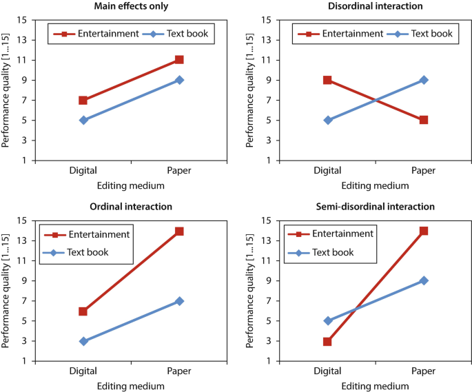
The original figure can be found here.

4.1.10 Which groups differ significantly?

The F-test only tells us that there is a significant difference exists, but it does not tell us which groups differ. Therefore, we need to conduct post-hoc tests or contrasts within a factor. Between the factors test pair comparisons can be conducted to check for significant differences.

4.1.11 Statistical assumptions

There are two assumptions for the ANOVA:

Normal distribution within the groups: dependent variable must be normally distributed in each group (but not necessarily in the overall sample)
Homogeneity of variance between groups: variances in the dependent variable must be the same in each group

The normal distribution assumption can be assessed visually. Furthermore, the Kolmogorov-Smirnov test (KS test) and Shapiro-Wilk test (more suitable from small samples < 50) can assess the distribution of the dependent variable against normal distribution, with deviations that are too large becoming significant (not desirable!). For serious violations of the normal distribution assumption:

the dependent variable can be normalized by transformations (e.g. logarithm, squaring, etc.)
problematic cases can be excluded
it is also possible to rely on a non-parametric analysis of variance (e.g. Kruskall-Wallis test)

Levene’s test can be used to test the null hypothesis that variances in the groups are equal (so rejecting this null hypothesis is undesirable). The analysis of variance (F-test) is quite robust against violations of the homogeneity of variance if the group sizes are (approximately) identical. However, post-hoc tests are not robust! In the case of serious violations of homogeneity of variance, there are two possibilities:

Correction of the F-ratio with Welch test (best choice)
Complete renunciation of F-test and calculation with Kruskall-Wallis test (non-parametric tests)

However, both are only possible with a one-factor analysis of variance! Therefore, as an approximation, it is possible to calculate the F-ratio for each factor individually using the Welch test and the Kruskall Wallis test. If the result is the same (sign. or not sign.), the result of the ANOVA can be trusted.

4.1.12 In a nutshell

ANOVA is based on the principle of scattering into explained and unexplained variance (F-test). In multi-factor ANOVA, variance is explained both by the individual factors and by their interaction (F-value for each factor and the interaction term).

\(Eta^2\) provides information about the effect size of the factors and interaction terms (compared to \(R^2\), which refers to the entire model).

There are different interaction types: ordinal, disordinal and semi-disordinal. The main effect of a factor can only be interpreted if it is not affected by a disordinal interaction.

Post-hoc tests show which factor levels differ significantly from each other. The Simple Effects Analysis shows for which factor levels of a factor A there is a significant difference due to factor B (interaction).

The ANOVA is based on two assumptions: normal distribution of the dependent variables and homogeneity of variances in the groups. It is generally quite robust to violations of these assumptions. There are tests to test these assumptions as well as procedures to report the results when they are violated.

4.2 Beyond one-way ANOVA

Below we explain the differences between the statistical methods ANOVA, ANCOVA, MANOVA, and MANCOVA.

4.2.1 ANCOVA

An ANCOVA (Analysis of Covariance) is also used to determine whether or not there is a statistically significant difference between the means of three or more independent groups. Unlike an ANOVA, however, an ANCOVA includes one or more covariates (CV), which can help us better understand how a factor impacts a response variable after accounting for some covariate(s).

Covariates are control variables whose influence on the dependent variable should be controlled. They are often variables that cannot be manipulated at all for theoretical or practical research reasons (e.g. age, gender, personality variables). They are included in the modeling as metric variables. Their influence on the dependent variable is calculated before the influence of the manipulated independent variables is calculated.

Covariates help us with reducing unexplained variance and within-group variance (SSE). The effect of the factors on the dependent variable can thus be determined more accurately (MSS). This improves the explanatory power of the overall model (\(R^2\)). The explanatory power of the factors (\(\eta^2\)) also improves.

The main advantage is that influences of other variables on the dependent variable can be “controlled” without being manipulated in the experiment. However, there are also disadvantages. For instance, the strict cause-and-effect logic of an experimental design does not apply to covariates. Futhermore, covariates must have a measurement (and they must be scale). Moreover, one can never include all relevant covariates. Note that we loses one degree of freedom of the residuals per covariate (SSE).

Example: political affiliation impacts on media coverage controlling for the number of social media followers (covariate).

4.2.2 ANCOVA assumptions

ANCOVA makes several assumptions about the data, such as:

Linearity between the covariate and the response variable at each level of the grouping variable.
- This can be checked by creating a clustered scatterplot of the covariate and the response variable.
Homogeneity of regression slopes: the slopes of the regression lines, formed by the covariate and the response variable, should be the same for each group.
- This can be verified visually as there should be no interaction between the outcome and the covariate (regression lines drawn by groups should be parallel).
The response variable should be approximately normally distributed.
- This can be verified using the Shapiro-Wilk normality test on the model residuals.
Homoscedasticity or homogeneity of variance of residuals for all groups.
- Residuals are assumed to have constant variance (homoscedasticity)
There should be no significant outliers within groups.

Nota bene: If several covariates are used, we also need low correlations between the covariates (avoidance of multicollinearity). In the case of multicollinearity, this would lead to a reduction of the degrees of freedom without a simultaneous reduction of the SS.

4.2.3 ANCOVA Post-hoc tests

“Normal” post-hoc tests cannot be called up for covariance analyses. However, there are three alternatives:

Post hoc tests on “estimated marginal means”
Contrasts
Simple effects analysis

4.2.4 MANOVA

A MANOVA (Multivariate Analysis of Variance) is identical to an ANOVA, except it uses two or more response variables. Similar to the ANOVA, it can also be one-way or two-way.

Example of one-way MANOVA: political affiliation impacts on media coverage and also on budget.

Example of two-way MANOVA: political affiliation and gender impact on media coverage and also on budget.

4.2.5 MANCOVA

A MANCOVA (Multivariate Analysis of Covariance) is identical to MANOVA, except it also includes one or more covariates. Similar to a MANOVA, a MANCOVA can also be one-way or two-way.

Example of one-way MANCOVA: political affiliation impacts on media coverage and also on budget while controlling for the number of social media followers (covariate).

Example of two-way MANCOVA: political affiliation and gender impact on media coverage and also on budget while controlling for the number of social media followers (covariate).

4.3 How it works in R?

See the lecture slides on one-way (M)AN(C)OVA:

You can also download the PDF of the slides here:

4.4 Quiz

True	False	Statement
		A p-value of .03 means that in only 3 in 100 times would a result as large as the one observed in a sample of data be observed if the null hypothesis were actually true for the population.
		A 2-way ANOVA compares the levels of two factors on a continuous variable.
		A covariate is a continuous independent variable in ANCOVA.
		In a 2-way MANCOVA, the 2 (or more) dependent variables should be unrelated.

My results will appear here

4.5 Example from the literature

The following article relies on ANOVA as a method of analysis:

Otto, L. P., Lecheler, S., & Schuck, A. R. (2020). Is context the key? The (non-) differential effects of mediated incivility in three European countries. Political Communication, 37(1), 88-107. Available here.

Please reflect on the following questions:

What is the research question of the study?
What are the research hypotheses?
Is ANOVA an appropriate method of analysis to answer the research question?
What are the main findings of the ANOVA analysis?

4.6 Time to practice on your own

You can download the PDF of the exercises here:

4.6.1 Exercice 1: ANOVA

We will be using the Gapminder data to see if the different continents really do have different life expectancy. In order to do this, we will perform an ANOVA using our continents as different groups, then test for differences between the groups.

Therefore, we would like to test the null hypothesis stating that there is no difference in the mean life expectancy between more continents (Europe, America, Asia, Africa, and Oceania). Let’s start by visualizing the differences using boxplots:

Show the code

data = gapminder::gapminder
ggpubr::ggboxplot(data, x = "continent", 
          y = "lifeExp", 
          color = "continent",
          ylab = "lifeExp", xlab = "continents")

Now, we want to formally compute ANOVA test:

Show the code

res.aov <- aov(lifeExp ~ continent, data = data)
summary(res.aov)
##               Df Sum Sq Mean Sq F value Pr(>F)    
## continent      4 139343   34836   408.7 <2e-16 ***
## Residuals   1699 144805      85                   
## ---
## Signif. codes:  0 '***' 0.001 '**' 0.01 '*' 0.05 '.' 0.1 ' ' 1

Interpretation

ANOVA tells us that continent does have a significant effect on life expectancy (F-value = 408.7 and p-value < 0.001). What we want now is to be able to tell what those differences are.

In ANOVA test, a significant p-value indicates that some of the group means are different, but we do not know which pairs of groups are different. To do so, we need to perform multiple pairwise-comparison:

Show the code

TukeyHSD(res.aov)
##   Tukey multiple comparisons of means
##     95% family-wise confidence level
## 
## Fit: aov(formula = lifeExp ~ continent, data = data)
## 
## $continent
##                       diff       lwr       upr     p adj
## Americas-Africa  15.793407 14.022263 17.564550 0.0000000
## Asia-Africa      11.199573  9.579887 12.819259 0.0000000
## Europe-Africa    23.038356 21.369862 24.706850 0.0000000
## Oceania-Africa   25.460878 20.216908 30.704848 0.0000000
## Asia-Americas    -4.593833 -6.523432 -2.664235 0.0000000
## Europe-Americas   7.244949  5.274203  9.215696 0.0000000
## Oceania-Americas  9.667472  4.319650 15.015293 0.0000086
## Europe-Asia      11.838783 10.002952 13.674614 0.0000000
## Oceania-Asia     14.261305  8.961718 19.560892 0.0000000
## Oceania-Europe    2.422522 -2.892185  7.737230 0.7250559

Interpretation

The output shows that Africa has a significantly lower life expectancy than every other continent, followed by Asia, and then the Americas. Oceania and Europe, meanwhile, have about equal life expectancy.

Remember that the ANOVA test assumes that, the data are normally distributed and the variance across groups are homogeneous. The residuals versus fits plot can be used to check the homogeneity of variances:

Show the code

plot(res.aov, 1)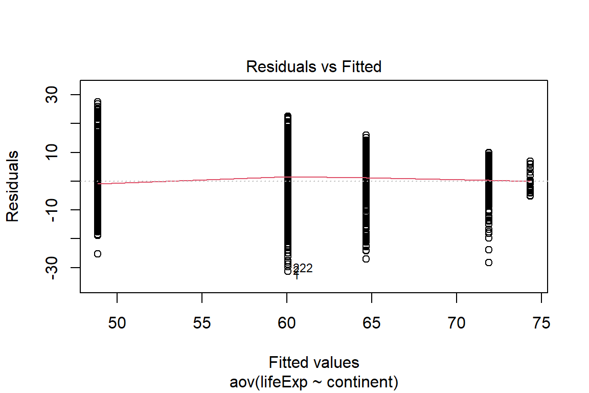

Interpretation

The plot shows no evident relationships between residuals and fitted values (the mean of each groups), which is good. So, we can assume the homogeneity of variances.

It is also possible to use Levene’ test (or Bartlett’s test) to check the homogeneity of variances (if the p-value is less than the significance level of 0.05, it means that there is evidence that the variance across groups is statistically significantly different):

Show the code

car::leveneTest(lifeExp ~ continent, data = data)
## Levene's Test for Homogeneity of Variance (center = median)
##         Df F value    Pr(>F)    
## group    4  51.568 < 2.2e-16 ***
##       1699                      
## ---
## Signif. codes:  0 '***' 0.001 '**' 0.01 '*' 0.05 '.' 0.1 ' ' 1

Interpretation

From the output of Levene’s test, we can see that the p-value is less than 0.05. This means that there is evidence to suggest that the variance across groups is statistically significantly different. Therefore, we cannot assume the homogeneity of variances.

The classical one-way ANOVA test requires an assumption of equal variances for all groups. An alternative procedure (Welch one-way test), that does not require that assumption have been implemented in the function oneway.test():

Show the code

oneway.test(lifeExp ~ continent, data = data)
## 
##  One-way analysis of means (not assuming equal variances)
## 
## data:  lifeExp and continent
## F = 664.9, num df = 4.00, denom df = 178.95, p-value < 2.2e-16
pairwise.t.test(data$lifeExp, data$continent,
                 p.adjust.method = "BH", pool.sd = FALSE)
## 
##  Pairwise comparisons using t tests with non-pooled SD 
## 
## data:  data$lifeExp and data$continent 
## 
##          Africa  Americas Asia    Europe
## Americas < 2e-16 -        -       -     
## Asia     < 2e-16 1.8e-08  -       -     
## Europe   < 2e-16 < 2e-16  < 2e-16 -     
## Oceania  < 2e-16 9.4e-14  < 2e-16 0.0064
## 
## P value adjustment method: BH

To test for the normality of residuals, we can plot the quantiles of the residuals against the quantiles of the normal distribution:

Show the code

plot(res.aov, 2)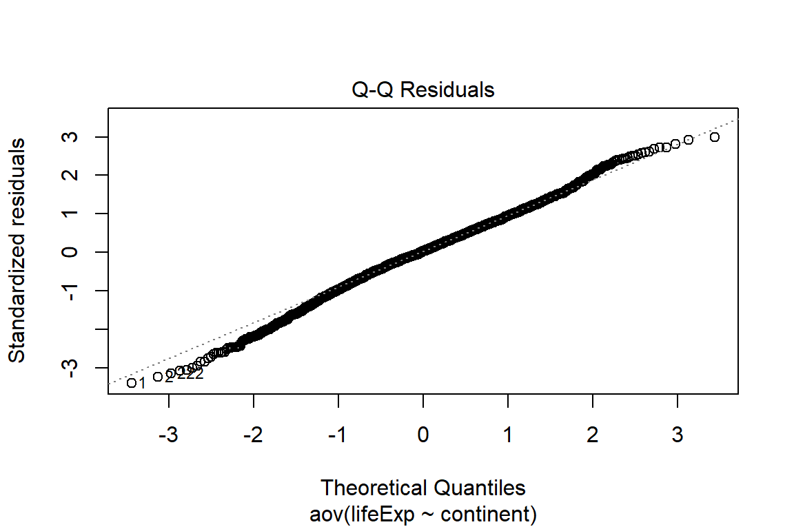

Interpretation

As all the points fall approximately along this reference line, we can assume normality.

The Shapiro-Wilk test on the ANOVA residuals can be used to assess whether normality is violated:

Show the code

aov_residuals <- residuals(object = res.aov)
shapiro.test(aov_residuals)
## 
##  Shapiro-Wilk normality test
## 
## data:  aov_residuals
## W = 0.9954, p-value = 0.000044

Interpretation

The Shapiro-Wilk test on the ANOVA residuals does not support the normality assumption.

A non-parametric alternative to one-way ANOVA is Kruskal-Wallis rank sum test, which can be used when ANOVA assumptions are not met:

Show the code

kruskal.test(lifeExp ~ continent, data = data)
## 
##  Kruskal-Wallis rank sum test
## 
## data:  lifeExp by continent
## Kruskal-Wallis chi-squared = 843.38, df = 4, p-value < 2.2e-16

4.6.2 Exercice 2: ANCOVA

In this exercise, you will learn how to:

Calculate and interpret one-way and two-way ANCOVA in R
Check ANCOVA assumptions
Perform post-hoc testing (multiple pairwise comparisons between groups to identify groups that are different)

For instance, we are interested in measuring the personalized style of campaigning (Y) explained by the political affiliation (X) and the available budget (CV). To do so, we will rely on the data covering the Swiss part of the Comparative Candidate Survey. We will be using the Selects 2019 Candidate Survey.

Let’s start by selecting the relevant variables and by recoding them (also select politicians with a budget equal or below CHF 50,000.-):

Show the code

library(foreign)
db <- read.spss(file=paste0(getwd(),
"/data/1186_Selects2019_CandidateSurvey_Data_v1.1.0.sav"), 
                use.value.labels = F, 
                to.data.frame = T)
sel <- db |>
  dplyr::select(B12,T9a,B6) |>
  stats::na.omit() |>
  dplyr::rename("budget"="B12",
                "party"="T9a",
                "personalization"="B6")
# budget without outliers
sel$budget <- as.numeric(as.character(sel$budget))
sel <- sel[sel$budget<=50000,]
# party recoded into left-center-right
sel$party_r <- NA
sel$party_r <- ifelse(sel$party==3 | 
                        sel$party==5, "1. left", as.character(sel$party_r))
sel$party_r <- ifelse(sel$party==2 | 
                        sel$party==6, "2. center", as.character(sel$party_r))
sel$party_r <- ifelse(sel$party==1 | 
                        sel$party==4, "3. right", as.character(sel$party_r))
sel <- sel[!is.na(sel$party_r),]
# personalization (invert scale)
sel$personalization <- as.numeric(as.character(sel$personalization))
sel$personalization <- (sel$personalization-10)*(-1)

Now, we can create a scatterplot between the covariate (budget) and the response variable (personalization), and add regression lines showing the equations and \(R^2\) by groups (party affiliations):

Show the code

p = ggpubr::ggscatter(
  sel, x = "budget", y = "personalization",
  color = "party_r", add = "reg.line", size=0
  )+
  ggpubr::stat_regline_equation(
    ggplot2::aes(label =  paste(..eq.label.., ..rr.label.., sep = "~~~~"),
                 color = party_r)
    )
plot(p)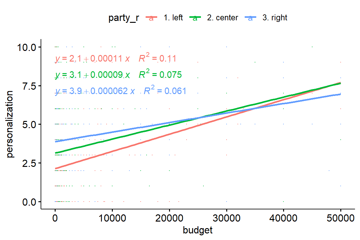

Interpretation

The figure displays a linear relationship between budget and personalization for each training party group.

Furthermore, we can see an interaction between the covariate and the independent variable (the party trends start to cross from a budget of ~25’000 Swiss francs). This violates the assumption of homogeneity of the regression slopes (there should be no significant interaction between the covariate and the grouping variable).

We can now verify whether there is a significant interaction between the covariate and the grouping variable:

Show the code

sel |> rstatix::anova_test(personalization ~ party_r*budget)
## ANOVA Table (type II tests)
## 
##           Effect DFn  DFd       F        p p<.05   ges
## 1        party_r   2 1382  39.858 1.48e-17     * 0.055
## 2         budget   1 1382 120.642 5.75e-27     * 0.080
## 3 party_r:budget   2 1382   3.434 3.30e-02     * 0.005

Interpretation

The output shows that there is no homogeneity of regression slopes as the interaction term is statistically significant (F(2, 1382) = 3.43, p = 0.005).

Nota bene: this does not mean that the model is “wrong” per se, as the fact that the interaction is significant tells us something interesting about the relationship between the variables.

Nota bene: The order of the variables is important in the calculation of the ANCOVA. You want to remove the effect of the covariate first and before entering your primary variable or interest:

Show the code

res.aov <- sel |> rstatix::anova_test(personalization ~ budget + party_r)
rstatix::get_anova_table(res.aov)
## ANOVA Table (type II tests)
## 
##    Effect DFn  DFd       F        p p<.05   ges
## 1  budget   1 1384 120.220 6.97e-27     * 0.080
## 2 party_r   2 1384  39.718 1.69e-17     * 0.054

Pairwise comparisons can be made to identify groups that are statistically different. Bonferroni’s multiple test correction is applied using the emmeans_test() function from the rstatix package:

Show the code

compa = sel |> 
  rstatix::emmeans_test(
    personalization ~ party_r, covariate = budget,
    p.adjust.method = "bonferroni"
    )
compa[,c(3,4,6,7)]
## # A tibble: 3 × 4
##   group1    group2    statistic        p
##   <chr>     <chr>         <dbl>    <dbl>
## 1 1. left   2. center     -6.04 1.93e- 9
## 2 1. left   3. right      -8.54 3.36e-17
## 3 2. center 3. right      -3.26 1.16e- 3

To estimate the normality of the residuals, you first need to calculate the model using lm(). In R, you can easily augment your data to add predictors and residuals using the function augment() from the broom package and then use the Shapiro-Wilk test.

Show the code

model <- lm(personalization ~ budget + party_r, data = sel)
model.metrics <- broom::augment(model) 
rstatix::shapiro_test(model.metrics$.resid)
## # A tibble: 1 × 3
##   variable             statistic  p.value
##   <chr>                    <dbl>    <dbl>
## 1 model.metrics$.resid     0.973 1.35e-15

Interpretation

The Shapiro Wilk test is significant (p < 0.001), so we cannot assume normality of residuals.

ANCOVA assumes that the variance of the residuals is equal for all groups. This can be checked using Levene’s test:

Show the code

model.metrics |> rstatix::levene_test(.resid ~ party_r)
## # A tibble: 1 × 4
##     df1   df2 statistic       p
##   <int> <int>     <dbl>   <dbl>
## 1     2  1385      6.70 0.00127

Interpretation

The Levene’s test is significant (p < 0.01), so we cannot assume homogeneity of the residual variances for all groups.

Furthermore, we need to check for outliers. These can be identified by looking at the normalized residuals (or studentized residuals), which is the residual divided by its estimated standard error. The normalized residuals can be interpreted as the number of standard errors outside the regression line.

Show the code

outliers = model.metrics |> 
  dplyr::filter(abs(.std.resid) > 3) |>
  as.data.frame()
outliers[,c(1:4,5:6,9)]
##   .rownames personalization budget party_r  .fitted   .resid     .cooksd
## 1      1696              10      0 1. left 2.229553 7.770447 0.005059324
## 2      1934              10    200 1. left 2.246654 7.753346 0.005000313