16 Latent Growth Modelling
16.1 Latent Growth Modelling (LGM)
LGM allows us to investigate longitudinal trends or group differences in measurement (also called growth trajectories). For example, suppose we want to model the political (or their political political engagement) polarization of panel participants over time. The objective of this chapter is to understand the concept of LGM and to be able to implement these models in lavaan.
16.2 Recap: lavaan syntax
Let’s first recall the typical lavaan syntax:
- ~ predict, used for regression of observed outcome to observed predictors
- =~ indicator, used for latent variable to observed indicator in factor analysis measurement models
- ~~ covariance
- ~1 intercept or mean (e.g., q01 ~ 1 estimates the mean of variable q01)
- 1* fixes parameter or loading to one
- NA* frees parameter or loading (useful to override default marker method)
- a* labels the parameter ‘a’, used for model constraints
- c(a,b)* specifically for multigroup models, see note below
16.3 Understanding the concept of LGM
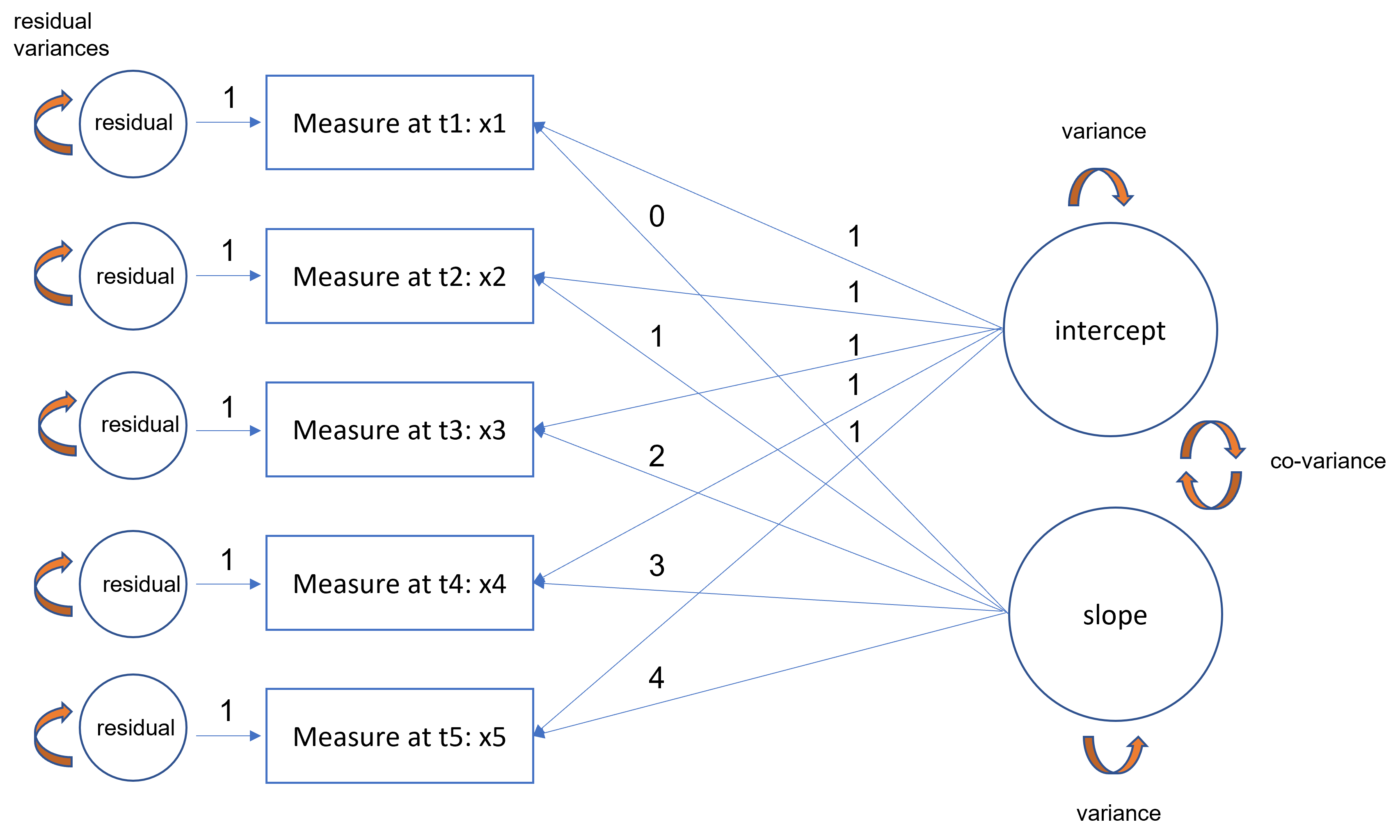
LGM are thus a special class of CFA models used to model trajectories over time. LGM models can be considered as an extension of the CFA model where the intercepts are freely estimated. Most commonly:
- the loadings for the intercept factor are all fixed to 1
- the loadings for the linear slope factor can be any ordered progression
- the first loading of the slope factor is fixed to 0
- the progression proceeds ordinally in increments of 1
- a one-unit increase in time is interpreted as an increase in the predicted outcome for a fixed time interval increase
Unlike traditional CFA models where the interpretation focuses on the loadings, the loadings are fixed in GLM which implies that the focus is on the latent intercept and linear slope factors.
For GLM, the dataset should be structured in wide format: each column represents the outcome (or dependent variable) at a specific time point. An assumption is that each observation or row must be independent of another. However, columns indicating outcomes are time dependent.
Here is a path diagram representing our particular LGM:

The equation for each time point defined for a person states as:
\[ x_{it} = \tau_{i} + \xi_{1} + (t)\xi_{2} + \delta_{it} \] where the observed intercepts are constrained to be zero (\(\tau_{i}=0\)). Furthermore, the (symmetric) variance covariance matrix of the latent intercept and slope is defined as:
\[ \Phi = \begin{bmatrix} \phi_{11}\\ \phi_{21} & \phi_{22} \end{bmatrix} \]
where \(\phi_{11}\) is the variance of the latent intercept, \(\phi_{22}\) is the variance of the latent slope and \(\phi{21}\) is the covariance of the intercept and slope. The population parameters correspond to the latent intercept and linear slope means.
16.4 Ordinal versus measured time in an LGM
The fixed loadings for the slope factor can be defined in different way depending on how time is modeled. For instance, it can be assumed that time is measured ordinally (in increments of year or semester), regardless of the actual measured time (the loadings will be 0,1,2,3,…). In other situations, it may be more beneficial to use measured time, such as for a study design where assessments are implemented at baseline, 3-, 6-, 9-, and 12-month follow-up (the loadings will be fixed at 0, 3, 6, 9 and 12), thus corresponding to the actual time of assessment. The choice of using ordinal versus measured time impacts on the mean of the intercept and slope and, therefore, the interpretation of these terms. A recommendation is that, if time intervals are unequal, it may be better to use measured time.
16.5 Quiz
| True | False | Statement |
|---|---|---|
| In a latent growth model, the observed intercepts are constrained to be zero but the latent intercepts are unconstrained to be free. | ||
| Suppose the mean of the slope is positive. A positive covariance between the intercept and slope means that for lower values of the starting X, the weaker the linear increase in X over time. | ||
| Suppose the last semester was four months long instead of three. If we continue to use ordinal time (i.e., 0,1,2,3,4), the mean of the slope factor would still be interpreted as the increase in X for every one semester increase in time. | ||
| Suppose the last semester was four months long instead of three. Using measured time would be more representative. |
16.6 Equivalence of the LGM to the hierarchical linear model (HLM)
LGM can be re-specified as an equivalent hierarchical linear model (HLM). The first modification is the format of the dataset: it should be in long format with repeated observations of time spanning multiple rows of data for every subject. For instance, HLM consists of repeated observations at Level 1 nested within individuals (index for time points: \(i\)) at Level 2 (index for individuals: \(j\)).
This suggests that the LGM model is equivalent to a HLM model with time nested within individuals with the following specifications:
- inclusion of a fixed effect of time at Level 1
- addition of a random intercept clustered by student and a random slope of time (indicated as time|student with the lmer syntax)
\[ y_{ij} = \beta_{0j} + \beta_{1j}*TIME_{ij} + r_{ij} \] \[ \beta_{0j} = \gamma_{00} + u_{0j} \] \[ \beta_{1j} = \gamma_{10} + u_{1j} \]
The important difference between the default LGM and HLM is that the residual variances of the LGM are unconstrained across timepoints but are constrained to be the same across time in a HLM by default. In order to constrain the residual variances in an LGM, we can use the a* notation in the lavaan syntax. In that case, the interpretation of the output is exactly the same for the LGM as it is for the HLM.
16.7 Adding a predictor to the LGM
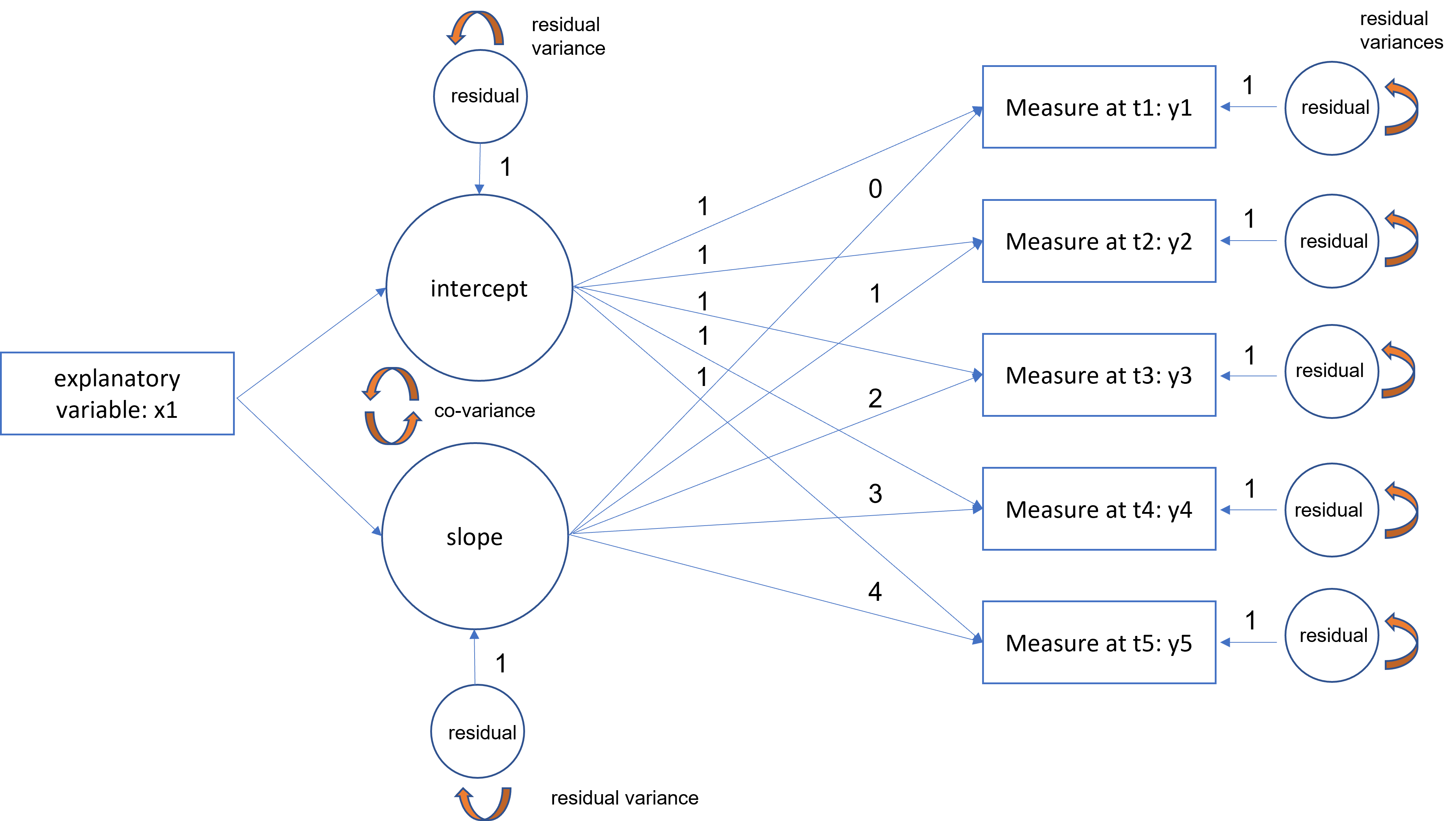
Until now, the fundamental latent growth model was characterized an intercept and linear growth factor, thus enabling us to answer the question of whether the linear trajectory is increasing, decreasing or flat over time. Now, we would like to find out what are potential predictors of this linear trajectory. For example, if the trajectory of political involvement increases over time, how does political affiliation predict this trend? Are there ideological differences in either the starting political involvement (intercept factor) or the growth trajectory (slope factor)? We thus would have the following specifications:
- latent factors now have a predictor
- latent intercept and slope factors become endogenous (y-side variables)
- there is a residual term which was not in the exogenous model (replace the variance of factor with the residual factor term)
- additional of an exogenous predictor (x1)

16.8 How it works in R?
See the lecture slides on LGM: