| Full Democ (N=24) |
Part Democ (N=52) |
Hybrid (N=39) |
Authoritarian (N=52) |
Overall (N=167) |
|
|---|---|---|---|---|---|
| literacy | |||||
| Mean (SD) | 100 (3) | 90 (10) | 70 (20) | 70 (20) | 80 (20) |
| Median [Min, Max] | 100 [80, 100] | 90 [40, 100] | 70 [20, 100] | 80 [30, 100] | 90 [20, 100] |
| Missing | 2 (8.3%) | 4 (7.7%) | 4 (10.3%) | 0 (0%) | 10 (6.0%) |
| pop_age | |||||
| Mean (SD) | 40 (4) | 30 (8) | 20 (7) | 20 (6) | 30 (9) |
| Median [Min, Max] | 40 [30, 40] | 30 [20, 40] | 20 [20, 40] | 20 [20, 40] | 30 [20, 40] |
| Missing | 0 (0%) | 1 (1.9%) | 0 (0%) | 0 (0%) | 1 (0.6%) |
| gender_unequal | |||||
| Mean (SD) | 0.3 (0.09) | 0.5 (0.2) | 0.7 (0.09) | 0.6 (0.1) | 0.5 (0.2) |
| Median [Min, Max] | 0.3 [0.2, 0.5] | 0.5 [0.2, 0.8] | 0.7 [0.5, 0.8] | 0.7 [0.4, 0.9] | 0.6 [0.2, 0.9] |
| Missing | 0 (0%) | 7 (13.5%) | 9 (23.1%) | 16 (30.8%) | 32 (19.2%) |
| religion | |||||
| Catholic | 12 (50.0%) | 24 (46.2%) | 8 (20.5%) | 8 (15.4%) | 52 (31.1%) |
| Orthodox Christian | 0 (0%) | 9 (17.3%) | 4 (10.3%) | 3 (5.8%) | 16 (9.6%) |
| Other Christian | 7 (29.2%) | 8 (15.4%) | 7 (17.9%) | 5 (9.6%) | 27 (16.2%) |
| Muslim | 0 (0%) | 4 (7.7%) | 14 (35.9%) | 28 (53.8%) | 46 (27.5%) |
| Buddhist | 1 (4.2%) | 2 (3.8%) | 4 (10.3%) | 4 (7.7%) | 11 (6.6%) |
| Other | 3 (12.5%) | 5 (9.6%) | 2 (5.1%) | 3 (5.8%) | 13 (7.8%) |
| Missing | 1 (4.2%) | 0 (0%) | 0 (0%) | 1 (1.9%) | 2 (1.2%) |
2 Quick recap: focus on bivariate statistics
2.1 Recap: bivariate statistic and hypothesis testing
When doing research, we go from the simplest to the most complex types of analysis. Each stage of the analysis brings information for the next step. However, this is an iterative process as sometimes it is necessary go back to simpler steps.
- Descriptive / univariate analysis
- Bivariate analysis
- Multivariate analysis (final model)
2.1.1 Univariate statistics
At the univariate stage, the objective is to become familiar with the variables (terms, missing data, atypical cases, etc.) and to propose a diagnosis of the variables (e.g. any filtering or recoding needed?). At this stage, we describe the distribution of observations over a variable (e.g. frequencies of all modalities of a variable) and we characterize the distribution of a variable (e.g. central tendency and dispersion) using appropriate tools (e.g. summaries, graphics, etc.).
2.1.2 Reporting descriptive statistics
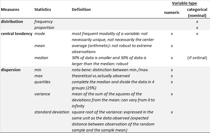
Below are some basic commands to calculate descriptive statistics. R provides packages/functions, which makes calculating and automatically generating a table of summary statistics for categorical and numeric variables. Let’s write an example with the “world” dataset from the “poliscidata” package by focusing on the following variables: dem_level4, literacy, pop_age, gender_unequal, religion. We will generate an example of a summary statistics table using the “table1” package. A full description of the dataset can be found here.
2.1.3 Fiability and validity
The Total Survey Error (TSE) framework (Biemer, 2010) accounts for the different sources of errors that occur at each stage of an investigation (e.g. coverage errors, selection errors, and measurement errors). Two important concepts are: reliability and validity. Reliability refers to the idea of replicability. It accounts for the degree of consistency of a measurement (by different observers, at different times). Validity addresses the conclusions we can draw from of a measure. For instance, internal validity aims at measuring the fit between the concept and the measure.
Sample statistics are estimators of population parameters. A particular point estimate cannot be expected to be exactly equal to the value of the parameter in the population. Therefore, the estimate always contains a margin of error. For instance, the normal law suggests that the distribution of a variable is around an average value and the other values increase and decrease in a homogeneous and symmetrical way around this average value. The distribution is thus in the form of a bell curve (or Gaussian curve).
The margin of error is also called the confidence interval. It corresponds to the area where we know for a given probability that the average or the percentage of a value will be found.
For a mean: \(\overline{x}\pm1.96(\frac{\sigma(X)}{\sqrt{n}})\)
where 1.96 represents the critical value from the standard normal distribution (depends on confidence level, e.g. 1.96 for 95%), \(\overline{x}\) is the mean, \(\sigma(X)\) is the population standard deviation, and \(n\) is the sample size.
For a proportion: \(Z_\alpha\sqrt{\frac{p(1-p)}{n}}\)
where \(Z_\alpha\) represents the critical value, \(p\) is the sample proportion, and \(n\) is the sample size.
2.1.4 Bivariate analysis
Inferential statistics makes use of probability theory. It indicates to the researcher the probability of being wrong by generalizing the findings of his study to the entire population, assuming a certain risk of error (generally 0.05, or 5%). To do so, two tools are used: estimation and hypothesis testing.
Three steps are generally applied:
- linking two variables: what values does DV take (e.g. use of social networks) according to an IV (e.g. political experience)?
- determining the statistical significance of this relationship (= hypothesis test)
- quantifying the strength of the relationship (and possibly determine its direction)
Statistical tools and tests in bivariate analysis depend on the level of measurement of the variables:
2.1.4.1 Relationship between two categorical variables
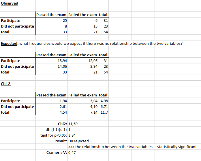
We can examine the relationship between two categorical variables based on a Chi-square test. The tested hypothesis reads as: what is the probability of obtaining the frequencies observed in the sample if there was no relationship between the two variables in the population? The null hypothesis states that the two variables are independent. The Chi-2 statistic is calculated as follows:
\[ Chi^2 = \sum{\frac{(o-e)^2}{e}} \]
where o is the observed value and e is the expected value.
This calculated Chi-2 statistic is compared to the critical value (obtained from statistical tables) with df=(r-1)(c-1) degrees of freedom and p = 0.05. If the calculated Chi-2 statistic is greater than the critical value, then the variables are not independent of each other and are, thus, significantly associated.
We can reproduce this example with R code:
Show the code
my_data=data.frame(passed=c(25,8),
                   failed=c(6,15))
rownames(my_data)=c("participated","not_participated")
chisq=chisq.test(my_data, correct = F) # No Yates correction (conservative)
round(chisq$expected,2)
##                  passed failed
## participated      18.94  12.06
## not_participated  14.06   8.94
chisq
##
##  Pearson's Chi-squared test
##
## data:  my_data
## X-squared = 11.686, df = 1, p-value = 0.0006297
2.1.4.2 Relationship between one interval variable and one categorical variable
We can compare the distribution of values on a quantitative variable (central tendency, dispersion) for different subpopulations (e.g. different modalities of the categorical independent variable). To see if the two variables are independent or if there is a relationship between them, we compare the variation between groups (mean) and the variation within groups (standard deviation). There is a relationship between two variables when the different groups are distinct and homogeneous.
We need to determine the statistical significance of the relationship to see if it can be generalized to the population. As for the crosstables, it is necessary to carry out a test of hypotheses. The null hypothesis states that the two variables are independent (if p<0.05 for the F-test, reject H0).
As with crosstables, there is also a measure of association: Eta ranging from 0 (perfect independence) to 1 (maximum association). In addition, Eta-2 informs us about the explanatory power of the model: percentage of the variance of the DV explained by the IV.
2.1.4.3 Relationship between two interval variables
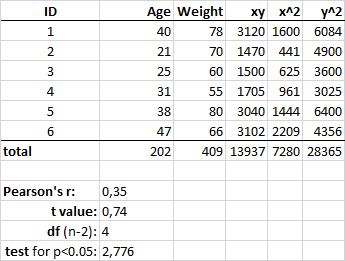
Correlation is a measure of association that provides information on the (linear) relationship between two quantitative variables, namely its direction and strength. The correlation coefficient, Pearson’s r, ranges from -1 (negative relationship) to +1 (positive relationship):
\[r = \frac{n\sum{xy}-\sum{x}\sum{y}}{\sqrt{(n\sum{x}^2-(\sum{x})^2)(n\sum{y}^2-(\sum{y})^2)}}\] The p-value can be determined by using the correlation coefficient table for the degrees of freedom (df = n−2) and calculating the t-value (and determining the corresponding p-value using the t-table):
\[ t = \frac{r}{\sqrt{1−r^2}}\sqrt{n-2} \]
If the p-value is < 5%, then the correlation between x and y is significant.
We can reproduce this example with R code:
Show the code
# install.packages("ggpubr")
# create a dataset
my_data <- data.frame(
  age=c(40,21,25,31,38,47),
weight=c(78,70,60,55,80,66))
# plot
ggpubr::ggscatter(my_data,
                  x = "age",
                  y = "weight",
          add = "reg.line",
          conf.int = TRUE,
          cor.coef = TRUE,
          cor.method = "pearson",
          xlab = "age", ylab = "weight")
# correlation test
cor.test(my_data$age,
         my_data$weight,
         method = "pearson")
##
##  Pearson's product-moment correlation
##
## data:  my_data$age and my_data$weight
## t = 0.74025, df = 4, p-value = 0.5002
## alternative hypothesis: true correlation is not equal to 0
## 95 percent confidence interval:
##  -0.6465987  0.9040106
## sample estimates:
##       cor
## 0.3471102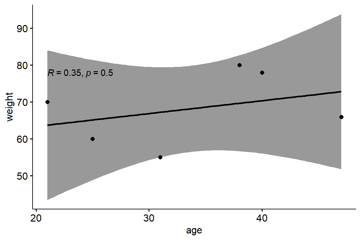
Nota bene: Do not forget to conduct preliminary test to check the test assumptions. In particular, is the covariation linear? Verify it using a scatter plot. Are the variables following a normal distribution? Use Shapiro-Wilk normality test using the function shapiro.test() and look at the normality plot using the function ggqqplot(). For the Shapiro-Wilk test, the null hypothesis states that the data are normally distributed.
2.2 How it works in R?
See the lecture slides on bivariate statistics:
2.3 Quiz
| True | False | Statement |
|---|---|---|
| Cross tabulation assesses the relationship between two variables with nominal measurement. | ||
| The p-value can be defined as the probability of observing a result when the null hypothesis is false. | ||
| The null hypothesis for the difference of means test posits that one group will have a higher average than another on the dependent variable. | ||
| It is important to assess the magnitude of the result whenever conducting a statistical test because a higher coefficient always means that it will be statistically significant. |
2.4 Time to practice on your own
2.4.1 Exercice 1: Poliscidata
2.4.1.1 Categorical × Categorical (Chi-square test)
Try to produce a crosstab in R between the variables standing for democratic decentralization (decent08) and the type of regime (dem_level4). What can you derive from the crosstab and its associated Chi-squared test? You can use the CrossTable() function from the descr package.
Show the code
db=poliscidata::world
db=db[,c("decent08","dem_level4")]
db$country = factor(db$decent08)
db$dem_level4 = factor(db$dem_level4)
descr::CrossTable(db$decent08, db$dem_level4, expected = F, chisq = T, prop.chisq = F)
##    Cell Contents
## |-------------------------|
## |                       N |
## |           N / Row Total |
## |           N / Col Total |
## |         N / Table Total |
## |-------------------------|
##
## ==========================================================================================
##                                   db$dem_level4
## db$decent08                       Full Democ   Part Democ   Hybrid   Authoritarian   Total
## ------------------------------------------------------------------------------------------
## No local elections                         0            3        4              16      23
##                                        0.000        0.130    0.174           0.696   0.202
##                                        0.000        0.097    0.160           0.432
##                                        0.000        0.026    0.035           0.140
## ------------------------------------------------------------------------------------------
## Lgsltr is elctd bt exctv is ap             5            7        5              14      31
##                                        0.161        0.226    0.161           0.452   0.272
##                                        0.238        0.226    0.200           0.378
##                                        0.044        0.061    0.044           0.123
## ------------------------------------------------------------------------------------------
## Lgsltr and exctv ar lclly elct            16           21       16               7      60
##                                        0.267        0.350    0.267           0.117   0.526
##                                        0.762        0.677    0.640           0.189
##                                        0.140        0.184    0.140           0.061
## ------------------------------------------------------------------------------------------
## Total                                     21           31       25              37     114
##                                        0.184        0.272    0.219           0.325
## ==========================================================================================
##
## Statistics for All Table Factors
##
## Pearson's Chi-squared test
## ------------------------------------------------------------
## Chi^2 = 30.41647 d.f. = 6 p = 0.0000328The Chi-squared test result indicates a statistically significant association between the type of local government elections and the level of democracy (p < 0.05). The observed distribution shows that countries without local elections are predominantly authoritarian, while those with both the legislature and executive locally elected are more likely to be full or partial democracies. The test’s Chi-squared value of 30.41647 with 6 degrees of freedom suggests that the differences in the distributions are unlikely to be due to random chance, pointing towards a meaningful relationship between local election practices and the overall level of democracy in a country.
Nota bene: The degrees of freedom (df) for a Chi-squared test are calculated based on the number of categories in the variables being analyzed. In this case, the degrees of freedom are 6. The formula for calculating degrees of freedom in a Chi-squared test for a contingency table is: \(df = (r−1)*(c−1) = (3−1)*(4−1) = 2*3 = 6\). The degrees of freedom determine which Chi-squared distribution to use for calculating the p-value. They reflect the complexity of the data and are used to compare the calculated Chi-squared value against the critical value from the Chi-squared distribution table to determine significance.
2.4.1.2 Interval × Binary Categorical (t-test)
Let’s now assess whether there is a statistically significant difference between the mean literacy level (literacy) and whether the government is a democracy (democ). You can rely on the t.test() function. What are your conclusions?
Show the code
db=poliscidata::world
db=db[,c("democ","literacy")]
db$country = factor(db$democ)
t.test(db$literacy ~ db$democ)
##
##  Welch Two Sample t-test
##
## data:  db$literacy by db$democ
## t = -3.4616, df = 138.73, p-value = 0.0007142
## alternative hypothesis: true difference in means between group No and group Yes is not equal to 0
## 95 percent confidence interval:
##  -17.593909  -4.801764
## sample estimates:
##  mean in group No mean in group Yes
## 74.12239 85.32022The Welch Two Sample t-test results indicate a statistically significant difference in literacy rates between countries categorized as “No” and “Yes” for democracy (p-value < 0.05). The test statistic (t = -3.4616) and degrees of freedom (138.73) support rejecting the null hypothesis, suggesting that the mean literacy rate is not equal between the two groups. Specifically, the mean literacy rate is lower in non-democratic countries (74.12) compared to democratic countries (85.32). The 95% confidence interval for the difference in means ranges from -17.59 to -4.80, further indicating that democratic countries tend to have significantly higher literacy rates.
We can also compare the difference between the means for a categorical variables with more than 2 categories. In this case, we use the ANOVA and the function aov(). Let’s compare the mean literacy level (literacy) for each type of regime (dem_level4). What are your conclusions?
Show the code
db=poliscidata::world
db=db[,c("dem_level4","literacy")]
db$country = factor(db$dem_level4)
summary(aov(db$literacy ~ db$dem_level4))
##                Df Sum Sq Mean Sq F value  Pr(>F)
## db$dem_level4   3  16942    5647   17.67 6.7e-10 ***
## Residuals     153  48900     320
## ---
## Signif. codes:  0 '***' 0.001 '**' 0.01 '*' 0.05 '.' 0.1 ' ' 1
## 10 observations deleted due to missingnessThe ANOVA results indicate a highly significant effect of the type of regime on literacy rates (F = 17.67, p < 0.05). With 3 degrees of freedom for the factor and 153 degrees of freedom for residuals, the results show that differences in types of regime are associated with significant variations in mean literacy rates.
2.4.1.3 Interval × Interval (Pearson correlation test)
Finally, let’s correlate the variables for literacy and Gender Inequality Index (gender_unequal). You can use the cor.test function. What is your conclusion?
Show the code
db=poliscidata::world
db=db[,c("gender_unequal","literacy")]
cor.test(db$gender_unequal, db$literacy, method=c("pearson"))
##
##  Pearson's product-moment correlation
##
## data:  db$gender_unequal and db$literacy
## t = -12.695, df = 126, p-value < 2.2e-16
## alternative hypothesis: true correlation is not equal to 0
## 95 percent confidence interval:
##  -0.81653 -0.66163
## sample estimates:
##        cor
## -0.7491485The Pearson’s product-moment correlation test results indicate a strong and statistically significant negative correlation between gender inequality and literacy rates (p-value < 0.05). The correlation coefficient (r = -0.749) suggests that higher levels of gender inequality are associated with lower literacy rates. The 95% confidence interval for the correlation ranges from -0.816 to -0.662, reinforcing the strength and direction of this relationship. The test statistic (t = -12.695) and degrees of freedom (126) further support the conclusion that the observed correlation is highly unlikely to be due to random chance, indicating a meaningful inverse relationship between these variables.
Nota bene: It is crucial to remember that correlation does not imply causation. This means that although gender inequality and lower literacy rates are related, we cannot conclude that one directly causes the other based solely on this correlation. Other factors could be influencing both variables. Establishing causation would require further research, including experimental or longitudinal studies to determine the direction and nature of the relationship.
2.4.2 Exercice 2: Gapminder
We will be using the Gapminder data to in the context of t-test, ANOVA and Chi-squared test. The goal is to train your understanding of the underlying principles of hypothesis testing and p-values (when to reject the null hypothesis or accept the alternative hypothesis when making inference about the population from sample data).
Let’s start by loading the Gapminder data and look at the mean life expectancy by countries:
Show the code
data = gapminder::gapminder
aggregate(lifeExp ~ continent, data, mean)
##   continent  lifeExp
## 1    Africa 48.86533
## 2  Americas 64.65874
## 3      Asia 60.06490
## 4    Europe 71.90369
## 5   Oceania 74.32621
Let’s presume that the mean life expectancy in Africa is 50 years old. We would like to test whether the observed mean from the sample (here: 48.86) is statistically different from the “true/presumed” mean:
Show the code
pop_mean=50 # according to H0
smp_mean=data$lifeExp[data$continent=="Africa"]
t.test(smp_mean, mu=pop_mean, alternative = "two.sided", conf.level = 0.95)
##
##  One Sample t-test
##
## data:  smp_mean
## t = -3.0976, df = 623, p-value = 0.002038
## alternative hypothesis: true mean is not equal to 50
## 95 percent confidence interval:
##  48.14599 49.58467
## sample estimates:
## mean of x
## 48.86533Here, we are testing a single sample against a known value. The results show that the sample mean (e.g., Africa) significantly differs from the presumed value (e.g., 50). The t-value is -3.09 and the associated p-value is 0.002. The confidence interval is given and does not contain the presumed value (e.g., 50).
Now, we would like to test the null hypothesis stating that there is no difference in the mean life expectancy between Europe and America:
Show the code
sub=data[data$continent=="Europe" | data$continent=="Americas",]
# visualize the distributions
ggplot2::ggplot(data=sub, ggplot2::aes(
  x=lifeExp, group=continent, fill=continent)) +
  ggplot2::geom_density(adjust=1.5, alpha=.4)
# conduct t.test
t.test(lifeExp ~ continent, data=sub, mu=0,
       alt="two.sided", conf=0.95, var.eq=F, paired=F)
##
##  Welch Two Sample t-test
##
## data:  lifeExp by continent
## t = -11.861, df = 460.72, p-value < 2.2e-16
## alternative hypothesis: true difference in means between group Americas and group Europe is not equal to 0
## 95 percent confidence interval:
##  -8.445287 -6.044612
## sample estimates:
## mean in group Americas   mean in group Europe
##               64.65874               71.90369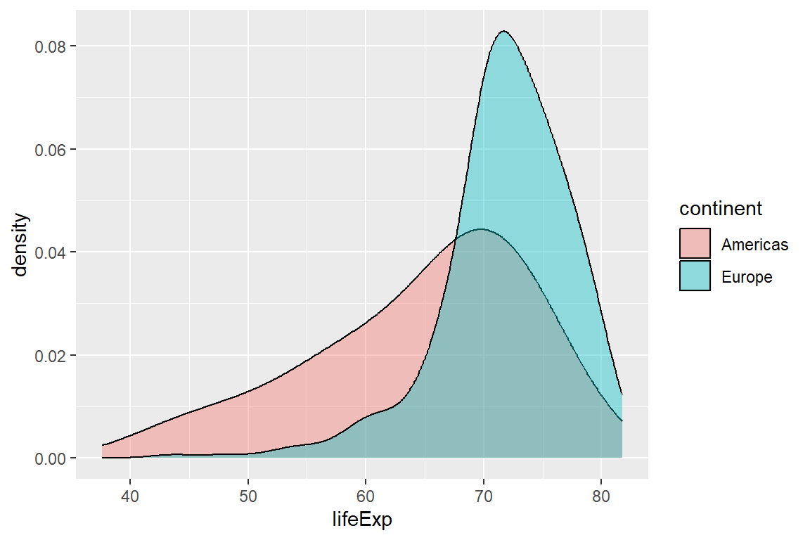
Here, we are comparing the mean life expectancy for two continents (e.g., Americas and Europe). The results show that there is a statistically significant difference in mean life expectancy between the continents (t-value = -11.86 and p-value < 0.001).
Now, we will add additional variables to the Gapminder data to test the relationship between levels of GDP and life expectancy. Start by creating two dichotomous variables (high vs low GDP and below vs above average life expectancy):
Show the code
library(plyr)
library(dplyr)
sel <- data %>%
  dplyr::filter(continent == "Europe") %>%
  plyr::mutate(gdp_factor = if_else(gdpPercap > mean(gdpPercap),
                              "high gdp", "low gdp"),
         below_avg_life_exp = if_else(lifeExp < mean(lifeExp),
         "low life expectancy", "high life expectancy"))
sel$gdp_factor <- as.factor(sel$gdp_factor)
sel$below_avg_life_exp <- as.factor(sel$below_avg_life_exp)
table(sel$gdp_factor, sel$below_avg_life_exp)
##
##            high life expectancy low life expectancy
##   high gdp                  134                  14
##   low gdp                    55                 157
Now, we want to look at the relationship between the two newly created dichotomous variables (high vs low GDP and below vs above average life expectancy). We can run a chi square test with the chisq.test() function:
Show the code
chisq.test(table(sel$gdp_factor, sel$below_avg_life_exp))
##
##  Pearson's Chi-squared test with Yates' continuity correction
##
## data:  table(sel$gdp_factor, sel$below_avg_life_exp)
## X-squared = 143.26, df = 1, p-value < 2.2e-16The chi square test shows a significant relationship between high vs low GDP and below vs above average life expectancy (chi square = 143.26 and p-value < 0.001).
Finally, we can look at the relationship between original variables for GDP and life expectancy using the cor.test() function:
Show the code
cor.test(data$lifeExp,data$gdpPercap)
##
##  Pearson's product-moment correlation
##
## data:  data$lifeExp and data$gdpPercap
## t = 29.658, df = 1702, p-value < 2.2e-16
## alternative hypothesis: true correlation is not equal to 0
## 95 percent confidence interval:
##  0.5515065 0.6141690
## sample estimates:
##       cor
## 0.5837062The correlation test shows a significant relationship between GDP and life expectancy (pearson = 0.58, t-value = 29.65 and p-value < 0.001). Note that most likely we would actually use a different correlation test, as the data on life expectancy are non-normal.
Optionally, a dynamic visualization is also possible using the following code:
Show the code
colors <- c('#C61951','#A4C6B0','#4AC6B7', '#1972A4', '#965F8A')
r3 <- plot_ly(
  data,
  x = ~gdpPercap,
  y = ~lifeExp,
  frame=~year,
  color = ~continent,
  type = "scatter",
  mode="markers",
  colors=~colors,
  size=~pop,
  marker = list(symbol = 'circle', sizemode = 'diameter',
                      line = list(width = 2, color = '#FFFFFF'), opacity=0.4)) %>%
  layout(
        title="Relationship between gdpPerCap and lifeExp over time",
        xaxis = list(title = 'gdpPercap',
                      # gridcolor = 'rgb(255, 255, 255)',
                      # range=c(10,50),
                      zerolinewidth = 1,
                      ticklen = 5,
                      gridwidth = 2),
         yaxis = list(title = 'lifeExp',
                      # gridcolor = 'rgb(255, 255, 255)',
                      # range=c(40,80),
                      zerolinewidth = 1,
                      ticklen = 5,
                      gridwith = 2),
        paper_bgcolor = 'rgb(243, 243, 243)',
        plot_bgcolor = 'rgb(243, 243, 243)'
  )%>%
  animation_opts(
    2000, redraw = FALSE
  ) %>%
  animation_slider(
    currentvalue = list(prefix = "YEAR ", font = list(color="black"))
  )
# r3
htmlwidgets::saveWidget(
                widget = r3, #the plotly object
                file = "images/PlotlyDynamic_GDPbyLifeExp.html",
                selfcontained = TRUE #creates a single html file
                )
2.5 DO IT YOURSELF
You can play with the R code and the gapminder dataset to train bivariate statistics. Click the “Run Code” button below to experience it and then try to add more code:
